The first goal for today is to define what we mean by temperature. In the process, we will discover that equilibrium is isothermal. That is, when two objects are in contact (so that they can exchange energy), then in equilibrium they have the same temperature. This is one of the big reasons why people care about temperature. It could be argued that the notion of temperature is constructed and defined in such a way as to guarantee that equilibrium is isothermal.
We follow the same approach as reference 39. See especially figure 3 therein. We shall use these ideas in section 14.4 and elsewhere.
In our first scenario, suppose we have two subsystems.
Each spin has −1 units of energy when it is in the down state and +1 units of energy when it is in the up state.
The two subsystems are able to exchange energy (and spin angular momentum) with each other, but the system as a whole is isolated from the rest of the universe.
Within limits, we can set up initial conditions with a specified amount of energy in each subsystem, namely E1 and E2. We can then calculate the entropy in each subsystem, namely S1 and S2. By considering various ways of distributing the energy and entropy, we can figure out which distribution corresponds to thermal equilibrium.
In particular, the subsystems reach equilibrium by exchanging energy with each other, under conditions of constant total energy E = E1 + E2. Therefore, at any given value of E, we can keep track of the equilibration process as a function of E1. We can calculate E2 as a function of E and E1. Then we can calculate everything else we need to know as a function of E1 and E2.
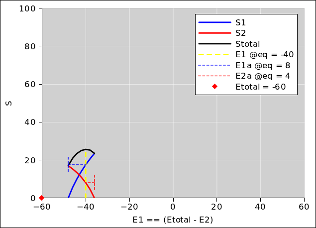
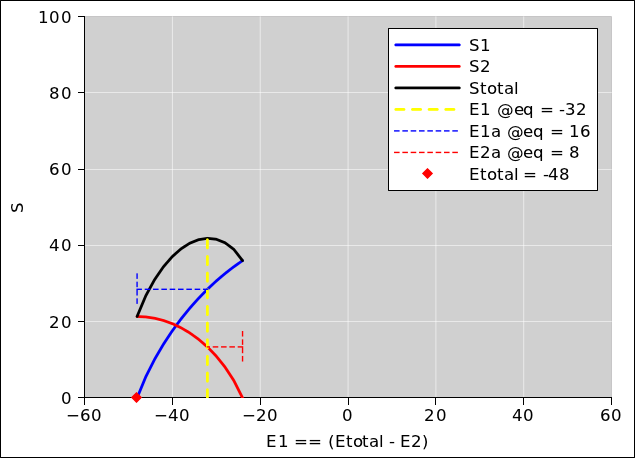
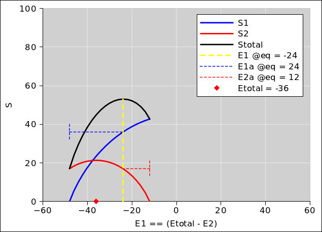
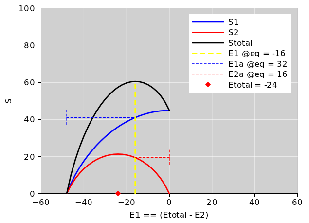
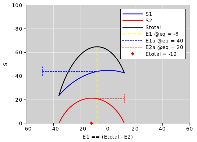
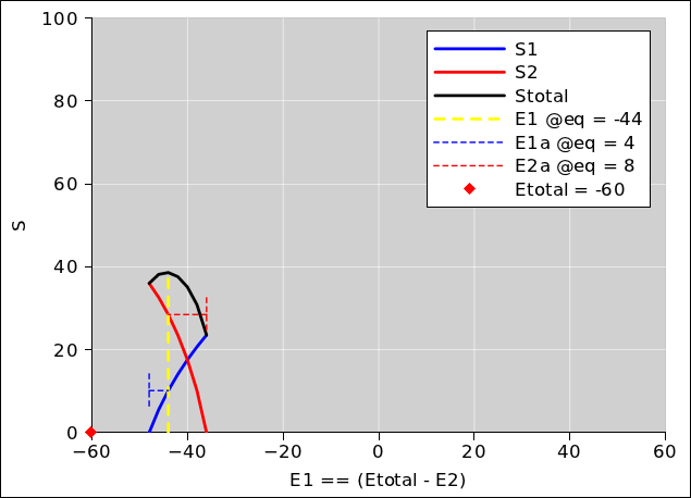
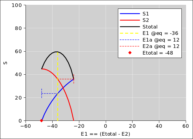
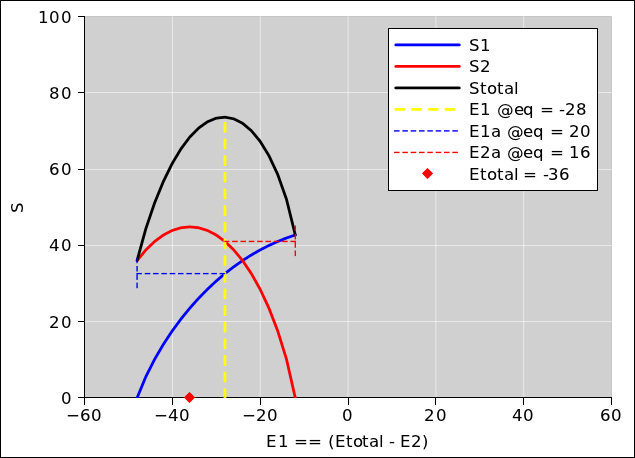
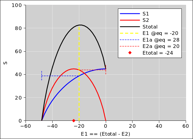
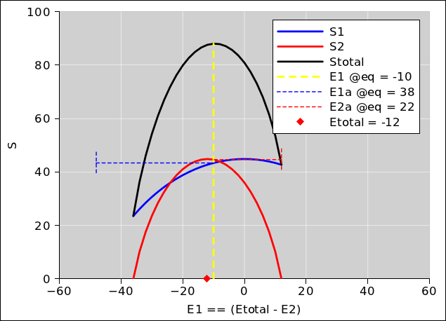
This equilibration process is diagrammed in figure 13.1, for the case where E = −60. Subsequent figures show the same thing for other amounts of energy. We pick eight different values for the total system energy, and calculate everything else accordingly. The method of calculation is discussed in section 13.5.
In each of the figures, there is quite a bit of information:
It is important to notice that the red curve plus the blue curve add up to make the black curve, everywhere. Therefore the slope of the red curve plus the slope of the blue curve add up to make the slope of the black curve, everywhere. At equilibrium, the slope of the black curve is zero, so the slope of the other two curves must be equal and opposite. You can see this in the graphs, at the places where the curves cross the yellow line.
For the blue curve, the slope is:
| (13.1) |
which depends only on properties of subsystem #1. As plotted in the figure, the slope of the red curve is ∂S2/∂E1, which is somewhat interesting, but in the long run we will be much better off if we focus attention on something that depends only on properties of subsystem #2, namely:
| (13.2) |
We now make use of the fact that the system is isolated, so that dE=0, and make use of conservation of energy, so that E = E1 + E2. Plugging this in to the definition of β2, we find
| (13.3) |
Therefore, when we observe that the slope of the blue curve and the slope of the red curve are equal and opposite, it tells us that β1 and β2 are just plain equal (and not opposite).
These quantitities are so important that the already has a conventional name: β1 is the inverse temperature of subsystem #1. Similarly β2 is the inverse temperature of subsystem #2.
The punch line is that when two subsystems have reached equilibrium by exchanging energy, they will be at the same temperature. We have just explained why this must be true, as a consequence of the definition of temperature, the definition of equilibrium, the law of conservation of energy, and the fact that the system is isolated from the rest of the world.
Experts note: The black curve measures ∂S/∂E1 not ∂S/∂E, so it cannot serve as a definition of temperature. Not even close. If we want to ascertain the temperature of the system, it usually suffices to measure the temperature of some subsystem. This is the operational approach, and it almost always makes sense, although it can get you into trouble in a few extreme cases. Hint: make sure there are at least two subsystems, each of which is big enough to serve as a heat sink for the other.
The remarks in this section apply only in the special case where one subsystem is twice as large as the other, and the two subsystems are made of the same kind of stuff. (The case where they are made of different stuff is more interesting, as discussed in section 13.3.)
You can see from the length of the horizontal dashed lines that at equilibrium, the blue subsystem has 2/3rds of the energy while the red subsystem has 1/3rd of the energy. This makes sense, since the blue system is twice as large, and the two subsystems are made of the same kind of stuff.
Meanwhile, you can see from the height of the horizontal dashed lines that at equilibrium, the blue subsystem has 2/3rds of the entropy while the red subsystem has 1/3rd of the entropy. Again this is unsurprising.
The vertical “tail” on the blue dashed line serves to indicate the E1 value that corresponds to E1a=0. Similarly, the vertical “tail” on the red dashed line serves to indicate the E1 value that corresponds to E2a=0.
Also, turning attention to E1 rather than E1a, you can see from the position of the yellow dashed line that E1 is 2/3rds of the total E, as shown by the red diamond, which represents total E even though it is plotted on the nominal E1 axis.
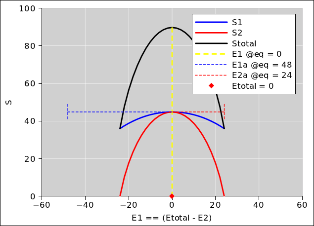
In this section we consider a new scenario. It is the same as the previous scenario, except that we imagine that the spins in the red subsystem have only half as much magnetic moment (or are sitting in half as much magnetic field). That means that the amount of energy that flips one spin in the blue subsystem will now flip two spins in the red subsystem.
We also double the number of spins in red subsystem, so that its maximum energy and minimum energy are the same as before.
Even though the red system cannot hold any more energy than it could before, it is now markedly more effective at attracting energy.
In this scenario, the two subsystems do not share the energy in a simple 1/3rd, 2/3rds fashion. At low temperatures, the red system is much more agressive than the blue system, and soaks up more than its “share” of the energy, more than you would have predicted based on its physical size or on the maximal amount of energy it could hold.
This illustrates an important point: All microstates are equally probable.
This stands in contrast to an oft-mentioned notion, namely the so-called principle of “equipartition of energy”. It is simply not correct to think that energy is equally distributed per unit mass or per unit volume or per atom or per spin. The fact is that probability (not energy) is what is getting distributed, and it gets distributed over microstates.
In the scenario considered in this section, the red system has more microstates, so it has more probability. As a consequence, it soaks up more energy, disproportionately more, as you can see by comparing the figures in this section with the corresponding figures in section 13.1. Be sure to notice the red and blue dashed horizontal lines.
In this scenario, equilibrium is isothermal ... as it must be, in any situation where subsystems reach equilibrium by exchanging energy. As a consequence, at equilibrium, the red slope and the blue slope are equal and opposite, as you can see in the diagrams.
It should be noted that temperature is not the same as energy. It’s not even the same as energy per unit volume or energy per unit mass. Dimensionally, it’s the same as energy per unit entropy, but even then it’s not the ratio of gross energy over gross entropy. In fact, temperature is the slope, namely T1 = ∂E1/∂S1|N1,V1.
That means, among other things, that constants drop out. That is to say, if you shift E1 by a constant and/or shift S1 by a constant, the temperature is unchanged.
As a specific example, suppose you have a box of gas on a high shelf and a box of gas on a low shelf. You let them reach equilibrium by exchanging energy. They will have the same temperature, pressure, et cetera. The box on the high shelf will have a higher gravitational potential energy, but that will not affect the equilibrium temperature at all.
By the same token, a wound-up spring will be in thermal equilibrium with an unstressed spring at the same temperature, and a charged-up capacitor will be in thermal equilibrium with an uncharged capacitor at the same temperature. The same goes for kinetic energy: A rapidly spinning flywheel will be in thermal equilibrium with a stationary flywheel at the same temperature. It’s not the energy that matters. It’s the slope ∂E/∂S that matters.
It is common knowledge that a parcel of air high in the atmosphere will be colder than a parcel of air at lower altitude. That tells us the atmosphere is not in thermal equilibrium. The temperature profile of the troposphere is more nearly adiabatic than isothermal, because it is vigorously stirred. Thunderstorms contribute quite a lot to the stirring, and it is no accident that the height of a typical thunderstorm is comparable to the altitude of the tropopause.
We can easily compute the spin entropy as a function of energy, using the obvious combinatoric formula.
| (13.4) |
Note that the binomial coefficient (
| ||
| It is implemented in typical spreadsheet programs by the combin(N,m) function. |
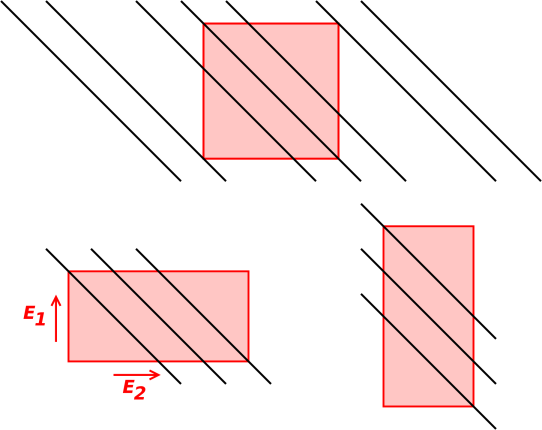
One tricky task is calculating the starting point and ending point of each of the curves in the diagrams. This task is not trivial, and can be understood with the help of figure 13.15. The colored rectangles represent the feasible ways in which energy can be allocated to the two subsystems. Each black line is a contour of constant total energy E, where E = E1 + E2. As you can see, depending on E and on the amount of energy that each subsystem can hold, there are at least 13 different ways in which the available energy can cross the boundaries of the feasible region.
By diagramming the task in this way, we reduce it to a problem in computer graphics, for which well-known solutions exist. It pays to code this systematically; otherwise you’ll spend unreasonable amounts of time debugging a bunch of special cases.
The spreadsheed used to produce the diagrams is available; see reference 40.
In this chapter we have demonstrated that
As we shall see in section 14.4, a closely parallel argument demonstrates that