See section 10.1 for an introduction to the fundamental concept of equilibrium.
See section 10.5 for an introduction to the fundamental concept of stability.
Suppose we have two objects that can interact with each other but are isolated from the rest of the universe. Object #2 starts out at a temperature T2, and we want to transfer some so-called “heat” to object #1 which starts out at some lesser temperature T1. We assume both temperatures are positive. As usual, trying to quantify “heat” is a losing strategy; it is easier and better to formulate the analysis in terms of energy and entropy.
Under the given conditions we can write
| (14.1) |
In more-general situations, there would be other terms on the RHS of such equations, but for present purposes we require all other terms to be negligible compared to the T dS term. This requirement essentially defines what we mean by heat transfer or equivalently thermal transfer of energy.
By conservation of energy we have
| (14.2) |
One line of algebra tells us that the total entropy of the world changed by an amount
| (14.3) |
or equivalently
| (14.4) |
From the structure of equation 14.4 we can see that entropy is created by a thermal transfer from the hotter object to the cooler object. Therefore such a transfer can (and typically will) proceed spontaneously. In contrast, a transfer in the reverse direction cannot proceed, since it would violate the second law of thermodynamics.
We can also see that:
A useful rule of thumb says that any reversible reversible thermal transfer will be rather slow. This can be understood in terms of the small temperature difference in conjunction with a finite thermal conductivity. In practice, people usually accept a goodly amount of inefficiency as part of the price for going fast. This involves engineering tradeoffs. We still need the deep principles of physics (to know what’s possible) ... but we need engineering on top of that (to know what’s practical).
Questions about equilibrium, stability, and spontaneity are often most conveniently formulated as maximization or minimization problems. This is not the most general way to do things, but it is a convenient and intuitive starting point. In the one-dimensional case especially, the graphical approach makes it easy to see what is going on.
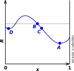
In figure 14.3, we are trying to minimize some objective function R (the “regret”). In an economics problem, R might represent the cost. In a physics or chemistry problem, R might represent something like the energy, or the Gibbs free enthalpy, or the negative of the entropy, or whatever. For now let’s just call it R.
In a physics problem, the abscissa x could be the position of a particle rolling in a potential well, subject to damping. In a chemistry problem, x could be the reaction coordinate, where x=0 corresponds to 100% reactants and x=1 corresponds to 100% products.
Global equilibrium corresponds to the lowest point on the curve. (If there are multiple points all at the minimum value, global equilibrium corresponds to this set of points.) This can be stated in mathematical terms as follows: For some fixed point A, if R(B) − R(A) is greater or equal to zero for all points B, then we know A is a global equilibrium point.
Note: Sometimes people try to state the equilibrium requirement in terms of ΔR, where ΔR := R(B)−R(A), but this doesn’t work very well. We are better off if we speak about point A and point B directly, rather than hiding them inside the Δ.
Now suppose we restrict point B to be near point A. Then if R(B) − R(A) is greater or equal to zero for all nearby points B, then we say A is a local equilibrium point. (A local equilibrium point may or may not be a global equilibrium point also.) In figure 14.3, point A is a global minimum, while point D is only a local minimum.
Now let’s consider the direction of spontaneous reaction. Given two points B and C that are near to each other, then if R(C) is less than R(B) then the reaction is will proceed in the direction from B to C (unless it is forbidden by some other law). In other words, the reaction proceeds in the direction that produces a negative ΔR.
Note that this rule applies only to small deltas. That is, it applies only to pairs of nearby points. In particular, starting from point B, the reaction will not proceed spontaneously toward point D, even though point D is lower. The local slope is the only thing that matters. If you try to formulate the rule in terms of ΔR in mathematical terms, without thinking about what it means, you will get fooled when the points are not nearby.
It is often interesting to ask whether a given situation is unstable, i.e. expected to change spontaneously – and if so, to ask in which direction it is expected to change. So, let’s examine what it means to talk about “direction” in thermodynamic state-space.
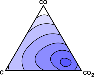
For starters, consider reactions involving carbon, oxygen, and carbon dioxide.
| C + O2 → CO2 (14.5) |
Under some conditions we have a simple reaction that proceeds mostly in the left-to-right direction equation 14.5, combining carbon with oxygen to form carbon dioxide. Meanwhile, under other conditions the reverse proceeds mostly in the opposite direction, i.e. the decomposition of carbon dioxide to form carbon and oxygen.
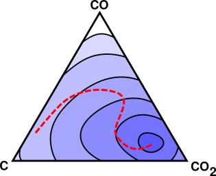
More generally, however, we need to consider other possibilities, such as the possible presence of carbon monoxide.
| (14.6) |
This is now a multi-dimensional situation, as shown schematically in figure 14.4.
Consider the contrast:
| In one dimension, we can speak of a given transformation proceeding forward or backward. Forward means proceeding left-to-right as written in equation 14.5, while backwards means proceeding right-to-left. | In multiple dimensions, we cannot speak of forward, backward, right, or left. We need to specify in detail what sort of step is taken when the transformation proceeds. |
Remark on terminology: In this document, the term “transformation” is meant to be very general, including chemical reactions and phase transitions among other things. (It is not necessary to distinguish “chemical processes” from “physical processes”.)
At any temperature other than absolute zero, a chemical reaction will never really go to completion. There will always be some leftover reactants and leftover intermediates, along with the nominal products. This is indicated by the contours in figure 14.4. The endpoint of the reaction is inside the smallest contour.
So far, in figure 14.3 and figure 14.4 we have been coy about what the objective function represents. Here’s a definite example: For an isolated system, the objective function is S, the entropy of the system. The endpoint is the point of maximum S, and we can interpret the contours in figure 14.4 as contours of constant S. As the reaction proceeds, it moves uphill in the direction of increasing S.
For a system that is not isolated – such as a system in contact with a heat bath – the system entropy S is not the whole story. The objective function is the entropy of the universe as a whole. Therefore we need to worry about not just the system entropy S, but also how much entropy has been pushed across the boundary of the system.
The ideas of section 14.1.4 and section 14.1.5 can be combined, as shown in figure 14.5. Sometimes a system is constrained to move along a lower-dimensional reaction pathway within a higher dimensional space.
Often it’s hard to know exactly what the pathway is. Among other things, catalysis can drastically change the pathway.
In all cases, the analysis is based on the second law of thermodynamics, equation 2.1, which we restate here:
| (14.7) |
We can use this to clarify our thinking about equilibrium, stability, reversibility, et cetera:
| (14.8) |
In other words, entropy is conserved during a reversible transformation.
| (14.9) |
In other words, entropy is created during a reversible transformation. You know the transformation is irreversible, because the reverse would violate the second law, equation 14.7.
To repeat: in all cases, we can analyze the system by direct application of the second law of thermodynamics, in the form given by equation 14.7. This is always possible, but not necessarily convenient.
Be that as it may, people really like to have an objective function. They like this so much that they often engineer the system to have a well-behaved objective function (exactly or at least approximately). That is, they engineer it so that moving downhill in figure 14.4 corresponds to creating entropy, i.e. an irreversible transformation. Moving along an isopotential contour corresponds to a transformation that does not create entropy, i.e. a reversible transformation.
Beware: This is tricky, because “the amount of entropy created” is not (in general) a function of state. Sometimes we can engineer it so that there is some function of state that tells us what we need to know, but this is not guaranteed.
Having an objective function is useful for multiple reasons. For one thing, it provides a way to visualize and communicate what’s going on. Also, there are standard procedures for using variational principles as the basis for analytical and computational techniques. These techniques are often elegant and powerful. The details are beyond the scope of this document.
You don’t know what the objective function is until you see how the system is engineered. In all cases the point of the objective function (if any) is to express a corollary to the second law of thermodynamics.
This completes the analysis of the general principle. The second law is the central, fundamental idea. However, direct application of the second law is often inconvenient.
Therefore the rest of this chapter is mostly devoted to developing less-general but more-convenient techniques. In various special situations, subject to various provisos, we can find quantities that are convenient to measure that serve as proxies for the amount of entropy created.
At this point we should discuss the oft-quoted words of David Goodstein. In reference 41, the section on “Variational Principles in Thermodynamics” begins by saying:
Fundamentally there is only one variational principle in thermodynamics. According to the Second Law, an isolated body in equilibrium has the maximum entropy that physics circumstances will allow.
The second sentence is true and important. For an isolated system, the maximum-entropy principle is an immediate corollary of the second law of thermodynamics, equation 14.7.
The first sentence in that quote seems a bit overstated. It only works if you consider a microcanonical (isolated) system to be more fundamental than, say, a canonical (constant-temperature) system. Note the contrast:
| The maximum entropy principle is not true in general; it is only true for an isolated system. | The second law of thermodynamics is true in all generality. |
The book goes on to say:
However, given in this form, it is often inconvenient to use.
It’s true that the maximum-entropy principle is often inconvenient, but it’s even worse than that. For a non-isolated system, maximizing the system entropy S is not even the correct variational principle. It’s not just inconvenient, it’s invalid. For a non-isolated system, in general there might not even be a valid variational principle of the type we are talking about.
In this section, we apply the general law to some important special cases. We derive some simplified laws that are convenient to apply in such cases.
Consider a completely isolated system. No entropy is flowing across the boundary of the system. If we know the entropy of the system, we can use that to apply the second law directly.
It tells us that the system entropy cannot decrease. Any transformation that leaves the system entropy unchanged is reversible, and any change that increases the system entropy is irreversible.
It must be emphasized that these conclusions are very sensitive to the provisos and assumptions of this scenario. The conclusions apply only to a system that isolated from the rest of the universe.
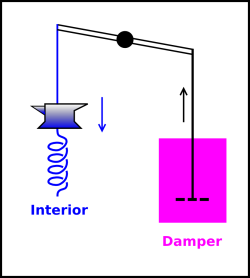
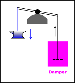
In figure 14.6, we have divided the universe into three regions:
The combination of interior region + neighborhood will be called the local region. We assume the local region is thermally isolated from the rest of the universe.
We have engineered things so that the linkage from the internal region to the damper to be thermally insulating. That means the internal region can do mechanical work on the damper, but cannot exchange entropy with it.
The decision to consider the damper as not part of the interior was a somewhat arbitrary, but not unreasonable. There are plenty of real-world systems where this makes sense, such as a charged harmonic oscillator (where radiative damping is not considered interior to the system) or a marble oscillating in a bowl full of fluid (where the viscous damping is not considered interior to the marble).
Local conservation of energy tells us:
| (14.10) |
We use unadorned symbols such as E and S etc. to denote the energy and entropy etc. inside the interior region. We use a subscript “n” as in En and Sn etc. to represent the energy and entropy etc. in the neighborhood. In this example, the neighborhood is the damper.
Now, suppose the oscillator starts out with a large amount of energy, large compared to kT. As the oscillator moves, energy will be dissipated in the damper. The entropy of the damper will increase. The entropy of the interior region is unknown and irrelevant, because it remains constant:
| (14.11) |
We require that the damper has some definite temperature. That allows us to relate its energy to its entropy in a simple way:
| (14.12) |
with no other terms on the RHS. There are undoubtedly other equally-correct ways of expanding dEn, but we need not bother with them, because equation 14.12 is correct and sufficient for present purposes.
Physically, the simplicity of equation 14.12 depends on (among other things) the fact that the energy of the neighborhood does not depend on the position of the piston within the damper (x), so we do not need an F·x term in equation 14.12. The frictional force depends on the velocity (dx/dt) but not on the position (x).
We assume that whatever is going on in the system is statistically independent of whatever is going on in the damper, so the entropy is extensive. Physically, this is related to the fact that we engineered the linkage to be thermally non-conducting.
| (14.13) |
Combining the previous equations, we find:
| (14.14) |
This means that for any positive temperature Tn, we can use the energy of the system as a proxy for the entropy of the local region.
So, let’s apply the second law to the local region. Recall that no entropy is flowing across the boundary between the local region and the rest of the universe. So the second law tells us that the system energy cannot increase. Any transformation that leaves the system energy unchanged is reversible, and any change that decreases the system energy is irreversible.
It must be emphasized that these conclusions are very sensitive to the provisos and assumptions of this scenario. The restrictions include: The system must be connected by a thermally-insulating linkage to a damper having some definite positive temperature, and the system must be isolated from the rest of the universe.
Another restriction is that the entropy within the system itself must be negligible or at least constant. If we implement the spring in figure 14.6 using a gas spring, i.e. a pneumatic cylinder, we would not be able to lower the system energy by condensing the gas, since that would require changing the system entropy.
Note: In elementary non-thermal mechanics, there is an unsophisticated rule that says “balls roll downhill” or something like that. That is not an accurate statement of the physics, because in the absence of dissipation, a ball that rolls down the hill will immediately roll up the hill on the other side of the valley.
If you want the ball to roll down and stay down, you need some dissipation, and we can understand this in terms of equation 14.14.
Note that the relevant temperature is the temperature of the damper, Tn. The system itself and the other non-dissipative components might not even have a well-defined temperature. The temperature (if any) of the non-dissipative components is irrelevant, because it doesn’t enter into the calculation of the desired result (equation 14.14). This is related to the fact that dS is zero, so we know TdS is zero even if we don’t know T.
In this section, we consider a different system, and a different set of assumptions.
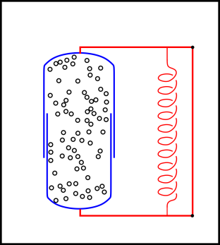
We turn our attention to a sample of gas, held under conditions of constant volume and constant positive temperature. We shall see that this allows us to answer questions about spontaneity using the system Helmholtz free energy F as a proxy for the amount of entropy created.
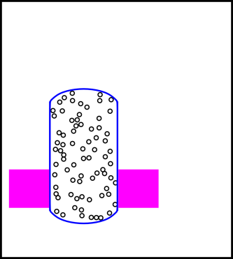
The situation is shown in figure 14.7. We have divided the universe into three regions:
The combination of interior region + neighborhood will be called the local region.
Inside the blue cylinder is some gas. In the current scenario, the volume of the cylinder is constant. (Compare this to the constant-pressure scenario in section 14.2.4, where the volume is not constant.)
Inside the neighborhood is a heat bath, as represented by the magenta region in the figure. It is in thermal contact with the gas inside the cylinder. We assume the heat capacity of the heat bath is very large.
We assume the combined local system (interior + neighborhood) is isolated from the rest of the universe. Specifically, no energy or entropy can flow across the boundary of the local system (the black rectangle in figure 14.7).
We use unadorned symbols such as F and S etc. to denote the free energy and entropy etc. inside the interior region. We use a subscript “n” as in En and Sn etc. to represent the energy and entropy etc. in the neighborhood.
Here’s an outline of the usual calculation that shows why dF is interesting. Note that F is the free energy inside the interior region. Similarly S is the entropy inside the interior region (in contrast to Slocal, which includes all the local entropy, Slocal = S + Sn). This is important, because it is usually much more convenient to keep track of what’s going on in the interior region than to keep track of everything in the neighborhood and the rest of the universe.
We start by doing some math:
| (14.15) |
Next we relate certain inside quantities to the corresponding outside quantities:
| (14.16) |
Next we assume that the heat bath is internal equilibrium. This is a nontrivial assumption. We are making use of the fact that it is a heat bath, not a bubble bath. We are emphatically not assuming that the interior region is in equilibrium, because one of the major goals of the exercise is to see what happens when it is not in equilibrium. In particular we are emphatically not going to assume that E is a function of S and V alone. Therefore we cannot safely expand dE = T dS − P dV in the interior region. We can, however, use the corresponding expansion in the neighborhood region, because it is in equilibrium:
| (14.17) |
Next, we assume the entropy is an extensive quantity. That is tantamount to assuming that the probabilities are uncorrelated, specifically that the distribution that characterizes the interior is uncorrelated with the distribution that characterizes the neighborhood. This is usually a very reasonable assumption, especially for macroscopic systems.
We are now in a position to finish the calculation.
| (14.18) |
This means that for any positive temperature Tn, we can use the Helmholtz free energy of the system as a proxy for the entropy of the local region.
So, let’s apply the second law to the local region. Recall that no entropy is flowing across the boundary between the local region and the rest of the universe. So the second law tells us that the system free energy cannot increase. Any transformation that leaves the system free energy unchanged is reversible, and any change that decreases the system free energy is irreversible.
It must be emphasized that these conclusions are very sensitive to the provisos and assumptions of this scenario. The conclusions apply only to a constant-volume system that can exchange energy thermally with a heat bath at some positive temperature ... and is otherwise isolated from the rest of the universe.
We now turn our attention to conditions of constant pressure and constant positive temperature. This is closely analogous to section 14.2.3; the only difference is constant pressure instead of constant volume. We shall see that this allows us to answer questions about spontaneity using the system’s Gibbs free enthalpy G as a proxy for the overall entropy Stotal.
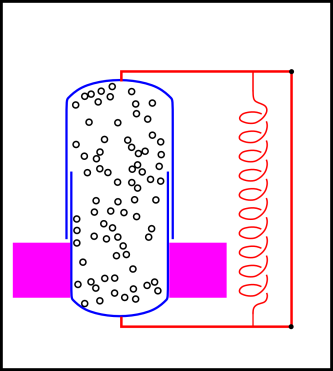
In figure 14.8, we have divided the universe into three regions:
The combination of interior region + neighborhood will be called the local region.
Inside the blue cylinder is some gas. The cylinder is made of two pieces that can slide up and down relative to each other, thereby changing the boundary between the interior region and the neighborhood. (Contrast this against the constant-volume scenario in section 14.2.3.)
Inside the neighborhood is a heat bath, as represented by the magenta region in the figure. It is in thermal contact with the gas inside the cylinder. We assume the heat capacity of the heat bath is very large.
Also in the neighborhood there is a complicated arrangement of levers and springs, which maintains a constant force (and therefore a constant force per unit area, i.e. pressure) on the cylinder.
We also assume that the kinetic energy of the levers and springs is negligible. This is a nontrivial assumption. It is tantamount to assuming that whatever changes are taking place are not too sudden, and that the springs and levers are somehow kept in thermal equilibrium with the heat bath.
We assume the combined local system (interior + neighborhood) is isolated from the rest of the universe. Specifically, no energy or entropy can flow across the boundary of the local system (the black rectangle in figure 14.8).
Note that G is the free enthalpy inside the interior region. Similarly S is the entropy inside the interior region (in contrast to Slocal, which includes all the local entropy, Slocal = S + Sn). This is important, because it is usually much more convenient to keep track of what’s going on in the interior region than to keep track of everything in the neighborhood and the rest of the universe.
We start by doing some math:
| (14.19) |
Next we relate certain inside quantities to the corresponding outside quantities. We will make use of the fact that in this situation, enthalpy is conserved, as discussed in section 14.3.2.
| (14.20) |
Next we assume that the heat bath is internal equilibrium. This is a nontrivial assumption. We are making use of the fact that it is a heat bath, not a bubble bath. We are emphatically not assuming that the interior region is in equilibrium, because one of the major goals of the exercise is to see what happens when it is not in equilibrium. In particular we are emphatically not going to assume that H is a function of S and P alone. Therefore we cannot safely expand dH = T dS + V dP in the interior region. However, we don’t need to do that. It suffices to rely on the assumption that the neighborhood is a well-behaved heat bath:
| (14.21) |
Again we assume the entropy is extensive. We are now in a position to finish the calculation.
| (14.22) |
So, let’s apply the second law to the local region. Recall that no entropy is flowing across the boundary between the local region and the rest of the universe. So the second law tells us that the system free enthalpy cannot increase. Any transformation that leaves the system free enthalpy unchanged is reversible, and any change that decreases the system free enthalpy is irreversible.
It must be emphasized that these conclusions are very sensitive to the provisos and assumptions of this scenario. The conclusions apply only to a constant-pressure system that can exchange energy thermally with a heat bath at some positive temperature ... and is otherwise isolated from the rest of the universe.
We now turn our attention to conditions of volume and constant positive temperature. The calculation is closely analogous to the previous sections. We shall see that this allows us to answer questions about spontaneity using the system’s enthalpy H as a proxy for the overall entropy Stotal.
In figure 14.9, the region inside the blue cylinder is insulated from the rest of the world. It cannot exchange energy with the rest of the world except insofar as it does mechanical work against the spring.
The cylinder is made of two pieces that can slide up and down relative to each other. Inside the cylinder is some gas. We call this the interior region.
In the neighborhood there is a complicated arrangement of levers and springs, which maintains a constant force (and therefore a constant force per unit area, i.e. pressure) on the cylinder.
There is no heat bath, in contrast to the constant-temperature scenario in section 14.2.4.
We also assume that the kinetic energy of the levers and springs is negligible. This is a nontrivial assumption. It is tantamount to assuming that whatever changes are taking place are not too sudden.
Note that H is the enthalpy inside the interior region. By definition, S is the entropy inside the interior region. In this scenario it is equal to the total entropy; that is, Stotal = S. That’s because there is no entropy in the neighborhood.
We start by doing some math:
| (14.23) |
The second law tells us that the system entropy cannot increase. Any transformation that leaves the system free enthalpy unchanged is reversible, and any change that decreases the system free enthalpy is irreversible.
It must be emphasized that these conclusions are very sensitive to the provisos and assumptions of this scenario. The conclusions apply only to a constant-pressure system that cannot exchange energy thermally with the rest of the universe.
Let’s take a moment to discuss a couple of tangentially-related points that sometimes come up.
In ultra-simple situations, it is traditional to divide the universe into two regions: “the system” versus “the environment”. Sometimes other terminology is used, such as “interior” versus “exterior”, but the idea is the same.
In more complicated situations, such as fluid dynamics, we must divide the universe into a great many regions, aka parcels. We can ask about the energy, entropy, etc. internal to each parcle, and also ask about the transfer of energy, entropy, etc. to adjacent parcels.
This is important because, as discussed in section 1.2, a local conservation law is much more useful than a global conservation law. If some energy disappears from my system, it does me no good to have a global law that says the energy will eventually reappear “somewhere” in the universe. The local laws says that energy is conserved right here, right now.
For present purposes, we can get by with only three regions: the interior, the immediate neighborhood, and the rest of the universe. Examples of this can be seen in section 14.2.3, section 14.2.4, and section 14.2.2.
Energy is always strictly and locally conserved. It is conserved no matter whether the volume is changing or not, no matter whether the ambient pressure is changing or not, no matter whatever.
Enthalpy is sometimes conserved, subject to a few restrictions and provisos. The primary, crucial restriction requires us to work under conditions of constant pressure.
Another look at figure 14.8 will help us fill in the details.
As always, the enthalpy is:
| (14.24) |
By conservation of energy, we have
| (14.25) |
Next we are going to argue for a “local conservation of volume” requirement. There are several ways to justify this. One way is to argue that it is corollary of the previous assumption that the local system is isolated and not interacting with the rest of the universe. Another way is to just impose it as a requirement, explicitly requiring that the volume of the local region (the black rectangle in figure 14.8) is not changing. A third way is to arrange, as we have in this case, that there is no pressure acting on the outer boundary, so for purposes of the energy calculation we don’t actually care where the boundary is; this would require extra terms in equation 14.27 but the extra terms would all turn out to be zero.
We quantify the idea of constant volume in the usual way:
| (14.26) |
Now we do some algebra:
| (14.27) |
Note that each of the calculations in section 14.2 was carried out by keeping track of the energy and entropy.
| Thinking in terms of energy and entropy is good practice. | Thinking in terms of “heat” and “work” would be a fool’s errand. |
| Energy is conserved. | Neither heat nor work is separately conserved. |
| We can easily understand that the linkage that connects the interior to the damper carries zero entropy and carries nonzero energy. | We see “work” leaving the interior in the form of PdV or F·dx. We see no heat leaving the interior. Meanwhile, we see heat showing up in the damper, in the form of TdS. This would be confusing, if we cared about heat and work, but we don’t care, so we escape unharmed. |
Keeping track of the energy and the entropy is the easy and reliable way to solve the problem.
Spontaneity is not quite the same as irreversibility, for the following reason: If a transformation can proceed in a direction that creates entropy, then as a rule of thumb, in many cases the transformation will spontaneously proceed in such a direction. However, this is only a rule of thumb, not a guarantee. As a counterexample, consider the transformation of diamond into graphite. Calculations show that under ordinary conditions this creates entropy, so it is definitely irreversible. However, the rate is so slow as to be utterly negligible, so we cannot say that the reaction occurs spontaneously, in any practical sense.
If a transformation does not occur, it might be because of the second law ... or because of any of the other laws of nature. It might be restricted by huge activation barriers, symmetries, selection rules, or other laws of physics such that it cannot create entropy at any non-negligible rate.
A reminder: The second law is only one law among many. Other laws include conservation of energy (aka the first law of thermodynamics), other conservation laws, various symmetries, spectroscopic selection rules, mathematical theorems, et cetera.
A process can proceed only if it complies with all the laws. Therefore if a process is forbidden by one of the laws, it is unconditionally forbidden. In contrast, if the process is allowed by one of the laws, it is only conditionally allowed, conditioned on compliance with all the other laws.
Based on a second-law analysis alone, we can determine that a process absolutely will not proceed spontaneously, in situations where doing so would violate the second law. In contrast, a second-law analysis does not allow us to say that a process “will” proceed spontaneously. Until we do a more complete analysis, the most we can say is that it might proceed spontaneously.
We are on much firmer ground when it comes to reversibility. In the context of ordinary chemical reactions, if we know the reaction can proceed in one direction, it is reversible if and only if it does not create entropy. That’s because of the reversibility of all the relevant1 fundamental laws governing such reactions, except the second law. So if there is no barrier to the forward reaction, there should be no barrier to the reverse reaction, other than the second law. (Conversely, if the reaction cannot proceed in any direction, because of conservation laws or some such, it is pointless to ask whether it is reversible.)
Consider the contrast:
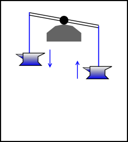
| In figure 14.10, there is no attempt to make the process reversible. The descent of the anvil is grossly dissipative. You can tell how much energy is dissipated during the process just by looking at the initial state and the final state. | In figure 14.11, the process is very nearly reversible. There will probably always be “some” friction, but we may be able to engineer the bearing so that the friction is small, maybe even negligible. Typically, to a good approximation, the power dissipation will be second order in the rate of the process, and the total energy dissipated per cycle will be first order in the rate. |
| We can call this “irreversible by state” and say that the amount of dissipation per operation is zeroth order in the rate (i.e. independent of the rate). | We can call this “irreversible by rate” and say that the amount of dissipation per operation is first order in the rate. |
|
| |
| Figure 14.10: Irreversible by State | Figure 14.11: Irreversible by Rate | |
In this section, we derive a couple of interesting results. Consider a system that is isolated from the rest of the universe, and can be divided into two parcels. We imagine that parcel #1 serves as a heat bath for parcel #2, and vice versa. Then:
We begin with a review of basic ideas of temperature in the equilibrium state, as introduced in chapter 13. With great generality, we can say that at thermodynamic equilibrium, the state of the system may change, but only in directions that do not create any entropy.
We write the gradient as dS rather than ∇S for technical reasons, but either way, the gradient is a vector. It is a vector in the abstract thermodynamic state-space (or more precisely, the tangent space thereof).
As usual, subject to mild conditions, we can expand dS using the chain rule:
| (14.28) |
We assume constant volume throughout this section. We also assume all the potentials are sufficiently differentiable.
We recognize the partial derivative in front of dE as being the inverse temperature, as defined by equation 24.4, which we repeat here:
| (14.29) |
We can rewrite the other partial derivative by applying the celebrated cyclic triple partial derivative rule:
| (14.30) |
For an explanation of where this rule comes from, see section 14.10. We can re-arrange equation 14.30 to obtain:
| (14.31) |
Note that if you weren’t fastidious about keeping track of the “constant E” “constant S” and “constant N” specifiers, it would be very easy to get equation 14.31 wrong by a factor of −1.
We recognize one of the factors on the RHS as the chemical potential, as defined by equation 7.32, which we repeat here:
| (14.32) |
Putting together all the ingredients we can write:
| (14.33) |
Since we can choose dN and dE independently, both terms on the RHS must vanish separately.
If we divide the system into two parcels, #1, and #2, then
| (14.34) |
plugging that into the definitions of β and µ, we conclude that at equilibrium:
| (14.35) |
The last two lines assume nonzero β i.e. non-infinite temperature.
So, we have accomplished the goal of this section. If/when the two parcels have reached equilibrium by exchanging energy, they will have the same inverse temperature. Assuming the inverse temperature is nonzero, then:
One way to visualize this is in terms of the gradient vector dS. The fact that dS=0 implies the projection of dS in every feasible direction must vanish, including the dE direction and the dN direction among others. Otherwise the system would be at non-equilibrium with respect to excursions in the direction(s) of non-vanishing dS.
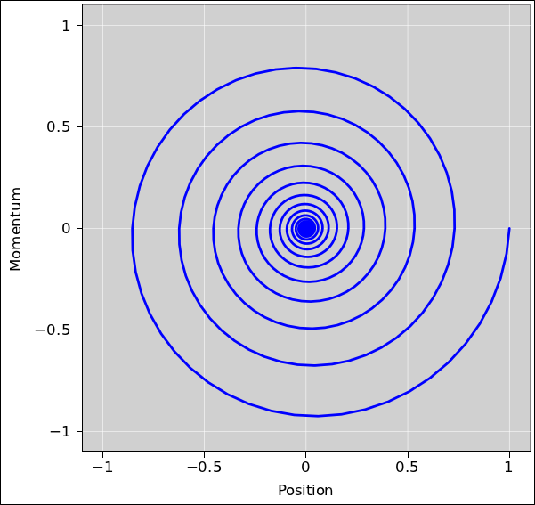
Figure 14.12 shows the position and momentum of a damped harmonic oscillator. The system starts from rest at a position far from equilibrium, namely (position, momentum) = (1, 0). It then undergoes a series of damped oscillations before settling into the equilibrium state (0, 0). In this plot, time is an implicit parameter, increasing as we move clockwise along the curve.
You will note that neither variable moves directly toward the equilibrium position. If we divide the phase space into quadrants, and look at the sequence of events, ordered by time:
This should convince you that the approach to equilibrium is not necessarily monotonic. Some variables approach equilibrium monotonically, but others do not.
When analyzing a complex system, it is sometimes very useful to identify a variable that changes monotonically as the system evolves. In the context of ordinary differential equations, such a variable is sometimes called a Lyapunov function.
In any physical system, the overall entropy (of the system plus environment) must be a monotone-increasing Lyapunov function, as we know by direct application of the second law of thermodynamics. For a system with external damping, such as the damped harmonic oscillator, decreasing system energy is a convenient proxy for increasing overall entropy, as discussed in section 14.2.2; see especially equation 14.14. Note that contours of constant energy are circles in figure 14.12, so you can see that energy decreases as the system evolves toward equilibrium.
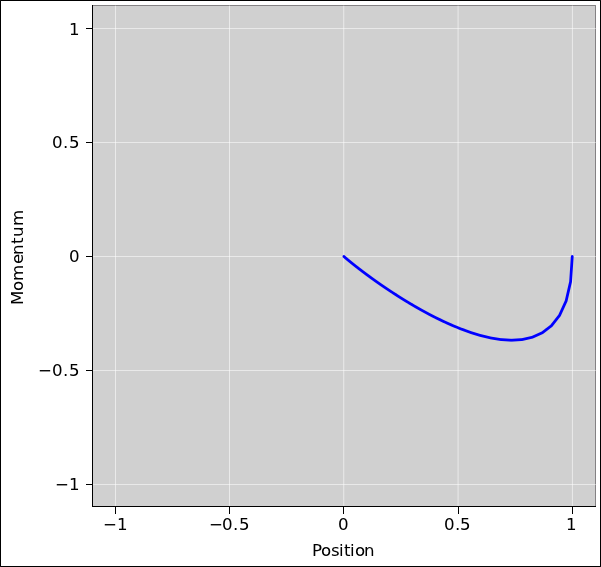
For a critically damped or overdamped system, the approach to equilibrium is non-oscillatory. If the system is initially at rest, the position variable is monotonic, and the momentum variable is “almost” monotonic, in the sense that its absolute value increases to a maximum and thereafter decreases monotonically. More generally, each variable can cross through zero at most once. The critically damped system is shown in figure 14.13.
We know that if two or more regions have reached equilibrium by the exchange of energy, they have the same temperature, subject to mild restrictions, as discussed in section 14.4. This is based on fundamental notions such as the second law and the definition of temperature.
We now discuss some much less fundamental notions:
Beware that some authorities go overboard and elevate these rules of thumb to the status of axioms. They assert that heat can never spontaneously flow from a lower-temperature region to a higher-temperature region. Sometimes this overstatement is even touted as “the” second law of thermodynamics.
This overstatement is not reliably true, as we can see from the following examples.
As a simple first example, consider a spin system. Region #1 is at a moderate positive temperature, while region #2 is at a moderate negative temperature. We allow the two regions to move toward equilibrium by exchanging energy. During this process, the temperature in region #1 will become more positive, while the temperature in region #2 will become more negative. The temperature difference between the two regions will initially increase, not decrease. Energy will flow from the negative-temperature region into the positive-temperature region.
This example tells us that the concept of inverse temperature is more fundamental than temperature itself. In this example, the difference in inverse temperature between the two regions tends to decrease. This is the general rule when two regions are coming into equilibrium by exchanging energy. It is a mistake to misstate this in terms of temperature rather than inverse temperature, but it is something of a technicality, and the mistake is easily corrected.
Here is another example that raises a much more fundamental issue: Consider the phenomenon of second sound in superfluid helium. The temperature oscillates like one of the variables in figure 14.12. The approach to equilibrium is non-monotonic.
Let’s be clear: For an ordinary material such as a hot potato, the equation of thermal conductivity is heavily overdamped, which guarantees that temperature approaches equilibrium monotonically ... but this is a property of the material, not a fundamental law of nature. It should not be taken as the definition of the second law of thermodynamics, or even a corollary thereof.
Suppose we assume, hypothetically and temporarily, that you are only interested in questions of stability, reversibility, and spontaneity. Then in this scenario, you might choose to be interested in one of the following thermodynamic potentials:
| (14.36) |
For more about these potentials and the relationships between them, see chapter 15.
There is nothing fundamental about the choice of what you are interested in, or what you choose to hold constant. All that is a choice, not a law of nature. The only fundamental principle here is the non-decrease of overall entropy, Stotal.
In particular, there is no natural or fundamental reason to think that there are any “natural variables” associated with the big four potentials. Do not believe any assertions such as the following:
|
I typeset equation 14.37 on a red background with skull-and-crossbones symbols to emphasize my disapproval. I have never seen any credible evidence to support the idea of “natural variables”. Some evidence illustrating why it cannot be generally true is presented in section 14.6.2.
Consider an ordinary heat capacity measurement that measures ΔT as a function of ΔE. This is perfectly well behaved operationally and conceptually.
The point is that E is perfectly well defined even when it is not treated as the dependent variable. Similarly, T is perfectly well defined, even when it is not treated as the independent variable. We are allowed to express T as T(V,E). This doesn’t directly tell us much about stability, reversibility, or spontaneity, but it does tell us about the heat capacity, which is sometimes a perfectly reasonable thing to be interested in.
Suppose we are interested in the following reaction:
| (14.38) |
which we carry out under conditions of constant pressure and constant temperature, so that when analyzing spontaneity, we can use G as a valid proxy for Stotal, as discussed in section 14.2.4.
Equation 14.38 serves some purposes but not all.
Let x represent some notion of reaction coordinate, proceeding in the direction specified by equation 14.38, such that x=0 corresponds to 100% reactants, and x=1 corresponds to 100% products.
Equation 14.38 is often interpreted as representing the largest possible Δx, namely leaping from x=0 to x=1 in one step.
That’s OK for some purposes, but when we are trying to figure out whether a reaction will go to completion, we usually need a more nuanced notion of what a reaction is. We need to consider small steps in reaction-coordinate space. One way of expressing this is in terms of the following equation:
| (14.39) |
where the parameters a, b, and c specify the “current conditions” and є represents a small step in the x-direction. We see that the RHS of this equation has been displaced from the LHS by an amount є in the direction specified by equation 14.38.
To say the same thing another way, equation 14.38 is the derivative of equation 14.39 with respect to x (or, equivalently, with respect to є). Equation 14.38 is obviously more compact, and is more convenient for most purposes, but you should not imagine that it describes everything that is going on; it only describes the local derivative of what’s going on.
The amount of free enthalpy liberated by equation 14.39 will be denoted δG. It will be infinitesimal, in proportion to є. If divide δG by є, we get the directional derivative ∇x G.
Terminology note: In one dimension, the directional derivative ∇x G is synonymous with the ordinary derivative dG/dx.
This tells us what we need to know. If ∇x G is positive, the reaction is allowed proceed spontaneously by (at least) an infinitesimal amount in the +x direction. We allow it to do so, then re-evaluate ∇x G at the new “current” conditions. If ∇x G is still positive, we take another step. We iterate until we come to a set of conditions where ∇x G is no longer positive. At this point we have found the equilibrium conditions (subject of course to the initial conditions, and the constraint that the reaction equation 14.38 is the only allowed transformation).
Naturally, if we ever find that ∇x G is negative, we take a small step in the −x direction and iterate.
If the equilibrium conditions are near x=1, we say that the reaction goes to completion as written. By the same token, if the equilibrium conditions are near x=0, we say that the reaction goes to completion in the opposite direction, opposite to equation 14.38.
Let’s consider the synthesis of ammonia:
| (14.40) |
We carry out this reaction under conditions of constant P and T. We let the reaction reach equilibrium. We arrange the conditions so that the equilibrium is nontrivial, i.e. the reaction does not go to completion in either direction.
The question for today is, what happens if we increase the pressure? Will the reaction remain at equilibrium, or will it now proceed to the left or right?
We can analyze this using the tools developed in the previous sections. At constant P and T, subject to mild restrictions, the reaction will proceed in whichever direction minimizes the free enthalpy:
| (14.41) |
where x is the reaction coordinate, i.e. the fraction of the mass that is in the form of NH3, on the RHS of equation 14.40. See section 14.2.4 for an explanation of where equation 14.41 comes from.
Note that P and T do not need to be constant “for all time”, just constant while the d/dx equilibration is taking place.
As usual, the free enthalpy is defined to be:
| G = E + PV − TS (14.42) |
so the gradient of the free enthalpy is:
| dG = dE + PdV − TdS (14.43) |
There could have been terms involving VdP and SdT, but these are not interesting since we are working at constant P and T.
In more detail: If (P1,T1) corresponds to equilibrium, then we can combine equation 14.43 with equation 14.41 to obtain:
| (14.44) |
To investigate the effect of changing the pressure, we need to compute
| (14.45) |
where P2 is slightly different from the equilibrium pressure; that is:
| P2 = (1+δ)P1 (14.46) |
We now argue that E and dE are insensitive to pressure. The potential energy of a given molecule depends on the bonds in the given molecule, independent of other molecules, hence independent of density (for an ideal gas). Similarly the kinetic energy of a given molecule depends on temperature, not on pressure or molar volume. Therefore:
| ⎪ ⎪ ⎪ ⎪ |
| = |
| ⎪ ⎪ ⎪ ⎪ |
| (14.47) |
Having examined the first term on the RHS of equation 14.45, we now examine the next term, namely the P dV/dx term. It turns out that this term is insensitive to pressure, just as the previous term was. We can understand this as follows: Let N denote the number of gas molecules on hand. Let’s say there are N1 molecules when x=1. Then for general x we have:
| N = N1 (2−x) (14.48) |
That means dN/dx = −N1, independent of pressure. Then the ideal gas law tells us that
| (P V) | ⎪ ⎪ ⎪ ⎪ |
| = |
| (N kT) | ⎪ ⎪ ⎪ ⎪ |
| (14.49) |
Since the RHS is independent of P, the LHS must also be independent of P, which in turn means that P dV/dx is independent of P. Note that the V dP/dx term is automatically zero.
Another way of reaching the same conclusion is to recall that PV is proportional to the kinetic energy of the gas molecules: PV = N kT = (γ−1) E, as discussed in section 26.5. So when the reaction proceeds left to right, for each mole of gas that we get rid of, we have to account for RT/(γ−1) of energy, independent of pressure.
This is an interesting result, because you might have thought that by applying pressure to the system, you could simply “push” the reaction to the right, since the RHS has a smaller volume. But it doesn’t work that way. Pressurizing the system decreases the volume on both sides of the equation by the same factor. In the PdV term, the P is larger but the dV is smaller.
Also note that by combining the pressure-independence of the dE/dx term with the pressure-independence of the P dV/dx term, we find that dH/dx is pressure-independent also, where H is the enthalpy.
Now we come to the −TdS/dx term. Entropy depends on volume.
By way of background, let us temporarily consider a slightly different problem, namely one that has only N1 molecules on each side of the equation. Consider what would happen if we were to run this new reaction backwards, i.e. right to left, i.e. from x=1 to x=0. The system volume would double, and we would pick up N1 k ln(2) units of entropy ... independent of pressure. It is the volume ratio that enters into this calculation, inside the logarithm. The ratio is independent of pressure, and therefore cannot contribute to explaining any pressure-related shift in equilibrium.
Returning to the main problem of interest, we have not N1 but 2N1 molecules when x=0. So when we run the real reaction backwards, in addition to simply letting N1 molecules expand, we have to create another N1 molecules from scratch.
For that we need the full-blown Sackur-Tetrode equation, equation 26.17, which we repeat here. For a pure monatomic nondegenerate ideal gas in three dimensions:
| (14.50) |
which gives the entropy per particle in terms of the volume per particle, in an easy-to-remember form.
For the problem at hand, we can re-express this as:
| (14.51) |
where the index i runs over the three types of molecules present (N2, H2, and NH3). We have also used the ideal gas law to eliminate the V dependence inside the logarithm in favor of our preferred variable P. We have (finally!) identified a contribution that depends on pressure and also depends on x.
We can understand the qualitative effect of this term as follows: The −TS term always contributes a drive to the left. According to equation 26.17, at higher pressure this drive will be less. So if we are in equilibrium at pressure P1 and move to a higher pressure P2, there will be a net drive to the right.
We can quantify all this as follows: It might be tempting to just differentiate equation 14.51 with respect to x and examine the pressure-dependence of the result. However, it is easier if we start by subtracting equation 14.44 from equation 14.45, and then plug in equation 14.51 before differentiating. A lot of terms are unaffected by the change from P1 to P2, and it is helpful if we can get such terms to drop out of the calculation sooner rather than later:
| (14.52) |
This quantitative result reinforces the previous qualitative analysis: If P2 is greater than P1, the reaction will proceed in the +x direction, since that is what will minimize G.
The calculation involved many steps, but each step was reasonably easy.
Remark: The result is surprisingly simple. Whenever a complicated calculation produces a simple result, it is a sign that we don’t really understand what’s going on. I suspect there is an easier way to obtain this result. In particular, since we have figured out that the entropy term is running the show, I conjecture that it may be possible to start from first principles and just keep track of the entropy.
Remark: In equation 14.52, by a first order expansion of the logarithm on the last line, you can verify that when the reaction is pushed toward equilibrium, the amount of push is proportional to δ, which makes sense.
Exercise: Use a similar argument to show that increasing the temperature will shift the equilibrium of equation 14.40 to the left. Hint: In a gas-phase reaction such as this, the side with more moles of gas will have more entropy.
One sometimes sees equilibrium (and or the shift of equilibrium) «explained» by reference to Le Châtelier’s «principle». This is highly problematic.
Le Châtelier in his lifetime gave two inconsistent statements of his so-called «principle». Restating them in modern terms:
Version 2 is tautological. As such, it is not wrong ... but it is utterly uninformative.
Version 1 is just wrong, as we can see from the following examples:
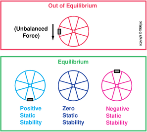
Example #1: As a familiar, important situation, consider ice in equilibrium with liquid water, under the usual constant-pressure conditions. Let x represent the reaction coordinate, i.e. the fraction of the mass of the system that is in the form of ice. If you perturb the system by changing x – perhaps by adding water, adding ice, or adding energy – the system will exhibit zero tendency to return to its previous x-value. This system exhibits zero stability, aka neutral instability, aka neutral stability, as defined in figure 14.2.
Example #2: Consider an equilibrium mixture of helium and neon. Let the reaction coordinate (x) be the fraction of the mass that is helium. If you perturb the system by increasing x, there will be no tendency for the system to react so as to decrease x. This is another example of zero stability aka neutral instability.
Example #3: Consider the decomposition of lead azide, as represented by the following reaction:
| (14.53) |
Initially we have x=0. That is, we have a sample of plain lead azide. It is in thermodynamic equilibrium, in the sense that it has a definite pressure, definite temperature, et cetera.
If we perturb the system by increasing the temperature a small amount, the system will not react so as to counteract the change, not even a little bit. Indeed, if we increase the temperature enough, the system will explode, greatly increasing the temperature.
We say that this system is unstable. More specifically, it exhibits negative stability, as defined in figure 14.2.
Example #4: Suppose you raise the temperature in an RBMK nuclear reactor. Do you think the reaction will shift in such a way as to counteract the increase? It turns out that’s not true, as some folks in Chernobyl found out the hard way in 1986.
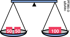
Example #5: A simple mechanical example: Consider a perfectly balanced wheel, as in the middle example in the bottom row of figure 14.2. It is in equilibrium. If you rotate it to a new angle, it will not exhibit any tendency to return to its original state. This is neutral stability, i.e. neutrally-stable equilibrium.
Example #6: Consider a wheel with an off-center weight at top dead center, as in the lower-right example in figure 14.2. It is in equilibrium, but it is unstable.
Suggestion: If you want to talk about equilibrium and stability, use the standard terminology, namely equilibrium and stability, as defined in figure 14.1 and figure 14.2. There is no advantage to mentioning Le Châtelier’s ideas in any part of this discussion, because the ideas are wrong. If you want to remark that “most” chemical equilibria encountered in the introductory chemistry course are stable equilibria, that’s OK ... but such a remark must not be elevated to the status of a “principle”, because there are many counterexamples.
Note that Lyapunov’s detailed understanding of what stability means actually predates Le Châtelier’s infamous «principle» by several years.
When first learning about equilibrium, stability, and damping, it is best to start with a one-dimensional system, such as the bicycle wheel depicted in figure 14.2. Then move on to multi-dimensional systems, such as an egg, which might be stable in one direction but unstable in another direction. Also note that in a multi-dimensional system, even if the system is stable, there is no reason to expect that the restoring force will be directly antiparallel to the perturbation. Very commonly, the system reacts by moving sideways, as discussed in section 14.5.
In this section, we derive a useful identity involving the partial derivatives of three variables. This goes by various names, including cyclic chain rule, cyclic partial derivative rule, cyclic identity, Euler’s chain rule, et cetera. We derive it twice: once graphically in section 14.10.1 and once analytically section 14.10.3. For an example where this rule is applied, see section 14.4.
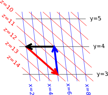
In figure 14.14 the contours of constant x are shown in blue, the contours of constant y are shown in black, and the contours of constant z are shown in red. Even though there are three variables, there are only two degrees of freedom, so the entire figure lies in the plane.
The red arrow corresponds to:
| (14.54) |
and can be interpreted as follows: The arrow runs along a contour of constant z, which is the z on the LHS of equation 14.54. The arrow crosses three contours of constant x, which is the numerator in equation 14.54. It crosses one contour of constant y, in the direction of decreasing y, which is the denominator.
Collecting results for all three vectors, we have:
| (14.55) |
and if we multiply those together, we get:
| (14.56) |
Note the contrast:
| The cyclic triple derivative identity is a topological property. That is, you can rotate or stretch figure 14.14 however you like, and the result will be the same: the product of the three partial derivatives will always be −1. All we have to do is count contours, i.e. the number of contours crossed by each of the arrows. | The result does not depend on any geometrical properties of the situation. No metric is required. No dot products are required. No notion of length or angle is required. For example, as drawn in figure 14.14, the x contours are not vertical, the y contours are not horizontal, and the x and y contours are not mutually perpendicular ... but more generally, we don’t even need to have a way of knowing whether the contours are horizontal, vertical, or perpendicular. |
Similarly, if you rescale one set of contours, perhaps by making the contours twice as closely spaced, it has no effect on the result, because it just increases one of the numerators and one of the denominators in equation 14.56.
The validity of equation 14.56 depends on the following topological requirement: The three vectors must join up to form a triangle. This implies that the contours {dx, dy, dz} must not be linearly independent. In particular, you cannot apply equation 14.56 to the Cartesian X, Y, and Z axes.
Validity also depends on another topological requirement: The contour lines must not begin or end within the triangle formed by the three vectors. We are guaranteed this will always be true, because of the fundamental theorem that says d(anything) is exact ... or, equivalently, d(d(anything)) = 0. In words, the theorem says “the boundary of a boundary is zero” or “a boundary cannot peter out”. This theorem is discussed in reference 4.
We apply this idea as follows: Every contour line that goes into the triangle has to go out again. From now on, let’s only count net crossings, which means if a contour goes out across the same edge where it came in, that doesn’t count at all. Then we can say that any blue line that goes in across the red arrow must go out across the black arrow. (It can’t go out across the blue arrow, since the blue arrow lies along a blue contour, and contours can’t cross.) To say the same thing more quantitatively, the number of net blue crossings inward across the red arrow equals the number of net blue crossings outward across the black arrow. This number of crossings shows up on the LHS of equation 14.56 twice, once as a numerator and once as a denominator. In one place or the other, it will show up with a minus sign. Assuming this number is nonzero, its appearance in a numerator cancels its appearance in a denominator, so all in all it contributes a factor of −1 to the product. Taking all three variables into account, we get three factors of −1, which is the right answer.
Here is yet another way of saying the same thing. To simplify the language, let’s interpret the x-value as “height”. The blue arrow lies along a contour of constant height. The black arrow goes downhill a certain amount, while the red arrow goes uphill by the same amount. The amount must be the same, for the following two reasons: At one end, the red and black arrows meet at a point, and x must have some definite value at this point. At the other end, the red and black arrows terminate on the same contour of constant x. This change in height, this Δx, shows up on the LHS of equation 14.56 twice, once as a numerator and once as a denominator. In one place or the other, it shows up with a minus sign. This is guaranteed by the fact that when the arrows meet, they meet tip-to-tail, so if one of the pair is pointed downhill, the other must be pointed uphill.
Let’s start over, and derive the result again. Assuming z can be expressed as a function of x and y, and assuming everything is sufficiently differentiable, we can expand dz in terms of dx and dy using the chain rule:
| (14.57) |
By the same token, we can expand dx in terms of dy and dz:
| (14.58) |
Using equation 14.58 to eliminate dx from equation 14.57, we obtain:
| (14.59) |
hence
| (14.60) |
We are free to choose dz and dy arbitrarily and independently, so the only way that equation 14.60 can hold in general is if the parenthesized factors on each side are identically zero. From the LHS of this equation, we obtain the rule for the reciprocal of a partial derivative. This rule is more-or-less familiar from introductory calculus, but it is nice to know how to properly generalize it to partial derivatives:
| (14.61) |
Meanwhile, from the parenthesized expression on the RHS of equation 14.60, with a little help from equation 14.61, we obtain the cyclic triple chain rule, the same as in section 14.10.1:
| (14.62) |
In this situation, it is clearly not worth the trouble of deciding which are the “independent” variables and which are the “dependent” variables. If you decide based on equation 14.57 (which treats z as depending on x and y) you will have to immediately change your mind based on equation 14.58 (which treats x as depending on y and z).
Usually it is best to think primarily in terms of abstract points in thermodynamic state-space. You can put your finger on a point in figure 14.14 and thereby identify a point without reference to its x, y, or z coordinates. The point doesn’t care which coordinate system (if any) you choose to use. Similarly, the vectors in the figure can be added graphically, tip-to-tail, without reference to any coordiate system or basis.
If and when we have established a coordinate system:
Note that there no axes in figure 14.14, strictly speaking. There are contours of constant x, constant y, and constant z, but no actual x-axis, y-axis, or z-axis.
In other, simpler situations, you can of course get away with a plain horizontal axis and a plain vertical axis, but you don’t want to become too attached to this approach. Even in cases where you can get away with plain axes, it is a good habit to plot the grid also (unless there is some peculiar compelling reason not to). Modern software makes it super-easy to include the grid.
For more on this, see reference 42.
In chemistry, the word “irreversible” is commonly used in connection with multiple inconsistent ideas, including:
Those ideas are not completely unrelated … but they are not completely identical, and there is potential for serious confusion.
You cannot look at a chemical reaction (as written in standard form) and decide whether it is spontaneous, let alone whether it goes to completion. For example, consider the reaction
| (14.63) |
If you flow steam over hot iron, you produce iron oxide plus hydrogen. This reaction is used to produce hydrogen on an industrial scale. It goes to completion in the sense that the iron is used up. Conversely, if you flow hydrogen over hot iron oxide, you produce iron and H2O. This is the reverse of equation 14.63, and it also goes to completion, in the sense that the iron oxide is used up.
What’s more, none of that has much to do with whether the reaction was thermodynamically reversible or not.
In elementary chemistry classes, people tend to pick up wrong ideas about thermodynamics, because the vast preponderance of the reactions that they carry out are grossly irreversible, i.e. irreversible by state, as discussed in section 14.3.6. The reactions are nowhere near isentropic.
Meanwhile, there are plenty of chemical reactions that are very nearly reversible, i.e. irreversible by rate, as discussed in section 14.3.6. In everyday life, we see examples of this, such as electrochemical reactions, e.g. storage batteries and fuel cells. Another example is the CO2/carbonate reaction discussed below. Alas, there is a tendency for people to forget about these reversible reactions and to unwisely assume that all reactions are grossly irreversible. This unwise assumption can be seen in the terminology itself: widely-used tables list the “standard heat of reaction” (rather than the standard energy of reaction), apparently under the unjustifiable assumption that the energy liberated by the reaction will always show up as heat. Similarly reactions are referred to as “exothermic” and “endothermic”, even though it would be much wiser to refer to them as exergonic and endergonic.
It is very difficult, perhaps impossible, to learn much about thermodynamics by studying bricks that fall freely and smash against the floor. Instead, thermodynamics is most understandable and most useful when applied to situations that have relatively little dissipation, i.e. that are nearly isentropic.
Lots of people get into the situation where they have studied tens or hundreds or thousands of reactions, all of which are irreversible by state. That’s a trap for the unwary. It would be unwise to leap to the conclusion that all reactions are far from isentropic … and it would be even more unwise to leap to the conclusion that “all” natural processes are far from isentropic.
Chemists are often called upon to teach thermodynamics, perhaps under the guise of a “P-Chem” course (i.e. physical chemistry). This leads some people to ask for purely chemical examples to illustrate entropy and other thermodynamic ideas. I will answer the question in a moment, but first let me register my strong objections to the question. Thermodynamics derives its great power and elegance from its wide generality. Specialists who cannot cope with examples outside their own narrow specialty ought not be teaching thermodynamics.
Here’s a list of reasons why a proper understanding of entropy is directly or indirectly useful to chemistry students.
Much of the significance of this story revolves around the fact that if we arrange the weights and springs just right, the whole process can be made thermodynamically reversible (nearly enough for practical purposes). Adding a tiny bit of weight will make the reaction go one way, just as removing a tiny bit of weight will make the reaction go the other way.
Now some interesting questions arise: Could we use this phenomenon to build an engine, in analogy to a steam engine, but using CO2 instead of steam, using the carbonate ↔ CO2 chemical reaction instead of the purely physical process of evaporation? How does the CO2 pressure in this system vary with temperature? How much useful work would this CO2 engine generate? How much waste heat? What is the best efficiency it could possibly have? Can we run the engine backwards so that it works as a refrigerator?
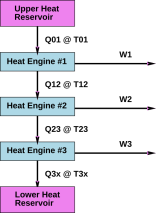
There are more questions of this kind, but you get the idea: once we have a reaction that is more-or-less thermodynamically reversible, we can bring to bear the entire machinery of thermodynamics.
To be really specific, suppose you are designing something with multiple heat engines in series. This case is considered as part of the standard “foundations of thermodynamics” argument, as illustrated figure 14.15. Entropy is conserved as it flows down the totem-pole of heat engines. The crucial conserved quantity that is the same for all the engines is entropy … not energy, free energy, or enthalpy. No entropy is lost during the process, because entropy cannot be destroyed, and no entropy (just work) flows out through the horizontal arrows. No entropy is created, because we are assuming the heat engines are 100% reversible. For more on this, see reference 8.