Hints on How to Do Math
John Denker
* Contents
-
1 Fundamental Suggestions
- 2 Multiple Methods of Solution
- 3 Drawing Inequalities
- 4 Long Multiplication
- 5 Long Division
- 6 Hindu Numeral System
- 7 Multiplying Multi-Term Expressions
- 8 Square Roots
-
8.1 Newton’s Method
- 8.2 First-Order Expansion
- 9 Simple Trig Functions
- 10 References
1 Fundamental Suggestions
Here are some hints on how to do basic math calculations.
These suggestions are intended to make your life easier. Some of them
may seem like extra work, but really they cause you less work in the
long run.
This is a preliminary document, i.e. a work in progress.
-
- 1.
Be tidy and systematic. Whenever you have data in tables,
especially when place-value is important, be sure to keep things
lined up in neat columns and neat rows. See section 4 for
an example of how this works in practice.
- 2.
If your columns are wobbly, get a pad of graph
paper and see if that helps. If you don’t have a supply of
store-bought graph paper, you can make graph paper on your computer
printer. There are freeware programs that do a very nice job of
this.
If that’s too much bother, start with a plain piece of paper and
sketch in faint guidelines when necessary.
- 3.
Paper is cheap. If you find that you are
running out of room on this sheet of paper, get another sheet of
paper, rather than squeezing the calculation into a smaller space.
See section 4 for an example of using extra paper to
achieve a better result.
- 4.
The whole calculation should be structured as a succession
of true statements. The first statement is true, the next statement
is true, and the statement after that, et cetera. Each statement is
a consequence of the previous statements (in conjunction with known
theorems, and the “givens” of the problem). Finally, we get to the
bottom line, and we know it is true. An example of this can be seen
in reference 1.
- 5.
Sometimes, especially for long and/or complex calculations, it
helps to organize your calculation in two columns. An example of
this can be seen in reference 1. In the left column, you
write an equation. In the right column, make a note as to how you
derived that equation. (Numbering all your equations makes this
easier.) If there isn’t enough width to do this easily, turn the
paper 90 degrees, so it becomes wider and less tall. (Writing paper
isn’t suitable for this, so use graph paper ... or lacking that,
plain white paper.)
- 6.
Avoid writing down an un-named number like 17, or an un-named
expression like a+17 ... because you might forget the meaning
thereof. Instead, whenever possible, write down an equation
such as b=a+17. That way you can point to every item on the page
and say that’s true, that’s true, that’s true... in accordance with
the strategy described in item 4.
- 7.
If the meaning of a variable-name such as a and b is
not obvious, construct a dictionary, glossary, or legend (like the
legend of a map) that explains in a sentence or two the meaning of
each variable. That is, a name is not the same as an explanation.
Do not expect the structure of a name or symbol to tell you
everything you need to know. Most of what you need to know belongs
in the legend. The name or symbol should allow you to look up the
explanation in the legend. For more on this, see the discussion of
names in reference 2.
Suppose the name is constructed according to a pattern, such as
FrT where F stands for force, the subscript r stands for
rolling resistance, and T stands for truck. In the glossary,
explain what each element means, so the reader doesn’t have to guess.
Does T stand for truck? Or does it stand for trailer? Or?????
- 8.
It is important to be able to go back and check the
correctness of the calculation you have done. See
section 4 and/or reference 1 for examples of
what this means in practice.
- 9.
As a corollary of item 8: Don’t perform
surgery on your equations. That is, once you write down a correct
equation, don’t start crossing out terms (or, worse, erasing terms)
and replacing them with other expressions. Such a substitution may
be “mathematically” correct, if the replacement is equal to the
thing being replaced ... but it is a bad strategy, because it makes
it hard for you to check your work. Instead, write a new equation.
Leave the old equation as it is. Paper is cheap. An example of this
can be seen in reference 1.
- 10.
Keep track of the units for each expression. For example,
the statement “x=2.5 inches” means something rather different
from “x=2.5 meters” ... and if you shorthand it as “x=2.5”
you’re just asking for trouble.
Sometimes the penalty for getting this wrong is 328 million dollars,
as in the case of the Mars Climate Orbiter
(reference 3).
 Figure 1
: Mars Climate Orbiter mission logo
Most computer languages do not automatically keep track of the units,
so you will have to do it by hand, in the comments. If the
calculation is nicely structured, it may suffice to have a
legend somewhere, spelling out the units for each of the
variables. If variables are re-used and/or converted from one set of
units to another, you need more than just a legend; you will need
comments (possibly quite a lot of comments) to indicate what units
are being used at each point in the code.
One policy that is sometimes helpful (but sometimes risky) is to
convert everything to SI units as soon as it is read in, even in
fields where SI units are not customary. Then you can do the
calculation in SI units and convert back to conventional units (if
necessary) immediately before writing out the results. (This is
problematic when writing an “intermediate” file. Should it be SI
or customary? How do you know the difference between an
“intermediate” result and a final result?)
It is certainly possible for computer programs to keep track of the
units automatically. A nice example is reference 4. It is
a shame that such features are not more widely available
- 11.
The factor-label method is a convenient and
powerful way of converting units when necessary. The correctness of
this method is a direct consequence of the axioms of algebra, since
it starts by multiplying by unity, which is allowed by the axioms.
- 12.
Haste makes waste, especially with multi-step processes. If
you work methodically, you’ll get the right answer the first time,
and that’s all there is to the story. If you try to do it twice as
fast, you’ll get the wrong answer, and then you’ll have to do it over
again ... and again ... and again.
2 Multiple Methods of Solution
Here’s a classic example: The task is to add 198 plus 215. The
easiest way to solve this problem in your head is to rearrange it as
(215 + (200 − 2)) which is 415 − 2 which is 413. The small point
is that by rearranging it, a lot of carrying can be avoided.
One of the larger points is that it is important to have multiple
methods of solution. This and about ten other important points are
discussed in reference 5.
3 Drawing Inequalities
The classic "textbook" diagram of an inequality uses shading to
distinguish one half-plane from the other. This is nice and
attractive, and is particularly powerful when diagramming the
relationship between two or more inequalities, as shown in
figure 2.
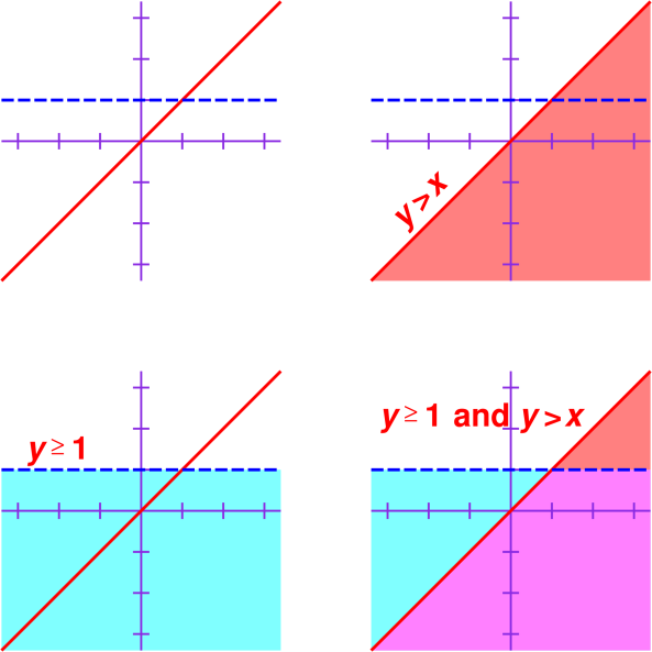 Figure 2
: Inequalities Represented using Shading
However, when you are working with pencil and paper, shading a
region is somewhere between horribly laborious and impossible.
It is much more practical to use hatching instead, as shown
in figure 3.
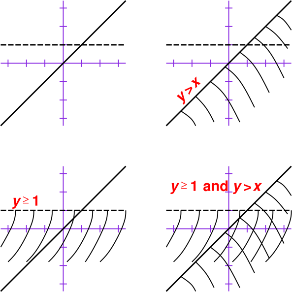 Figure 3
: Inequalities Represented using Hatching
Obviously the hatched depiction is not as beautiful as the shaded depiction,
but it is good enough. It is vastly preferable on cost/benefit
grounds, for most purposes.
Some refinements:
- I recommend hatching the excluded half-plane, so that the
solution-set remains unhatched rather than hatched. This is
particularly helpful when constructing the conjunction (logical
AND) of multiple inequalities.
- I recommend using solid lines versus dashed lines to distinguish
“≥” inequalities from “>” inequalities. If you’re going to
hatch the excluded half-plane, use solid lines for the “>”
inequalities, to show that the boundary itself is excluded.
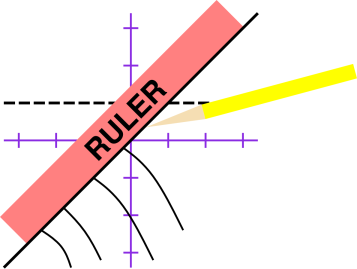
- As suggested in figure 4, for linear
inequalities you can do the hatching faster and more accurately with
the help of a ruler or straightedge, which makes it easy to ensure
that none of the hatches stray into the wrong region.
4 Long Multiplication
See reference 6.
5 Long Division
See reference 7.
6 Hindu Numeral System
The modern numeral system is based on place value. As we understand
it today, each numeral can be considered a polynomial in powers of
b, where b is the base of the numeral system. For decimal
numerals, b=10. As an example:
|
2468 | | = | | 2 b3 | + | 4 b2 | + | 6 b1 | + | 8 b0 |
| | | = | | 2000 | + | 400 | + | 60 | + | 8
|
| (1)
|
As discussed in reference 6, this allows us to
understand long multiplication in terms of the more general rule for
multiplying polynomials.
7 Multiplying Multi-Term Expressions
Given two expressions such as (a+b+c) and (x+y), each of which has
one or more terms, the systematic way to multiply the expressions is
to make a table, where the rows correspond to terms in the first
expression, and the rows correspond to terms in the second expression:
| | | | | | | | | | | |
| a | | | ax | | ay | |
| b | | | bx | | by | |
| c | | | cx | | cy | |
| |
|
| (a+b+c) · (x+y) | | = | | ax + ay + bx + by + cx + cy
|
| (2)
|
In the special case of multiplying a two-term expression by another
two-term expression, the mnemonic FOIL applies. That stands for
First, Outer, Inner, Last. As shown in figure 5, we start with
the First contribution, i.e. we multiply the first term from in each
of the factors. Then we add in the Outer contribution, i.e. the first
term from the first factor times the last term from the last factor.
Then we add in the Inner contribution, i.e. the last term from the
first factor times the first term from the last factor. Finally we
add in the Last contribution, i.e. we multiply the last terms from
each of the factors.
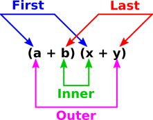 Figure 5
: FOIL = First + Outer + Inner + Last
8 Square Roots
8.1 Newton’s Method
If you can do long division, you can do square roots.
Most square roots are irrational, so they cannot be represented
exactly in the decimal system. (Decimal numerals are, after all,
rational numbers.) So the name of the game is to find a decimal
representation that is a sufficiently-accurate approximation.
We start with the following idea: For any nonzero x we know that
x÷√x is equal to √x. Furthermore, if s1 is
greater than √x it means x/s1 is less than √x. If
we take the average of these two things, s1 and x/s1, the
average is very much closer to √x. So we set
and then iterate. The method is very powerful; the number of digits
of precision doubles each time. It suffices to use a rough estimate
for the starting point, s1. In particular, if you are seeking the
square root of an 8-digit number, choose some 4-digit number as the
s1-value.
This is a special case of a more general technique called
Newton’s method, but if that doesn’t mean anything to you, don’t
worry about it.
8.2 First-Order Expansion
Note that the square of 1.01 is very nearly 1.02. Similarly, the
square of 1.02 is very nearly 1.04. Turning this around, we find the
general rule that if x gets bigger by two percent, then √x
gets bigger by one percent ... to a good approximation.
We can illustrate this idea by finding the square root of 50. Since
50 is 2% bigger than 49, the square root of 50 is 1% bigger than 7
... namely 7.07. This is a reasonably good result, accurate to better
than 0.02%.
If we double this result, we get 14.14, which is the square root of
200. That is hardly surprising, since we remember that the square
root of 2 is 1.414, accurate to within roundoff error.
9 Simple Trig Functions
Sine and cosine are transcendental functions. Evaluating them will
never be super-easy, but it can be done, with reasonably decent
accuracy, with relatively little effort, without a calculator.
In particular:
- You can always start with a zeroth-order approximation: For
angles near zero, the sine will be near zero. For angles near
90∘, the sine will be near 1. For angles near 30∘, the sine
will be near 0.5, et cetera.
- You can draw a graph, using the anchor points in equation 4 as a guide. You can then use graphical interpolation to
obtain values for any angle.
- A simple Taylor series gives a result accurate to 2.1% or
better using only a couple of multiplications. Remember to express
the angle in radians before using these formulas.
The following facts serve to “anchor” our knowledge of the sine
and cosine:
|
| |
| |
sin(0∘) | | = | | | | = | | 0 | | = | | cos(90∘) | | |
(4a)
|
|
| |
sin(30∘) | | = | | | | = | | 0.5 | | = | | cos(60∘) | | |
(4b)
|
|
| |
sin(45∘) | | = | | | | = | | 0.70711 | | = | | cos(45∘) | | |
(4c)
|
|
| |
sin(60∘) | | = | | | | = | | 0.86603 | | = | | cos(30∘) | | |
(4d)
|
|
| |
sin(90∘) | | = | | | | = | | 1 | | = | | cos(0∘) | | |
(4e)
|
| | |
|
Actually, that hardly counts as “remembering” because if you ever
forget any part of equation 4 you should be able to
regenerate it from scratch. The 0∘ and 90∘ values are
trivial. The 30∘ is a simple geometric construction. Then the
60∘ and 45∘ values are obtained via the Pythagorean theorem.
The value for 45∘ should be particularly easy to remember,
since √2 = 1.414 and √½ = ½√2.
The rest of this section is devoted to the Taylor series. A low-order
expansion works well if the point of interest is not too far from the
nearest anchor.
- For angles between −10∘ and +10∘, the approximation
sin(x)≈x is accurate to better than 0.51%. This is a
one-term Taylor series. Let’s call it the Taylor[1] approximation.
It is super-easy to evaluate, since it involves no additions and no
multiplications, or at most one multiplication if we need to convert
to radians from degrees or some other unit of measure. See
equation 5c and the blue line near x=0 in figure 6.
- For angles from 25∘ to 65∘, all the points are with a
few degrees of one of the anchor points in equation 4.
This means the first-order Taylor series is accurate to better than 1
percent in this region. We can call this the Taylor[0,1]
approximation. It requires knowing the sine and the cosine at the
nearest anchor point ... which we do in fact know from equation 4. See equation 9 and the blue line in
figure 6.
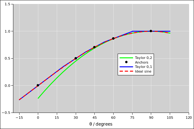 Figure 6
: Piecewise 1st-Order Taylor Approximation to Sine
- For a rather broad range of angles near the top of the sine,
from 65∘ to 115∘, the approximation sin(x)≈1−x2/2
is accurate to better than half a percent. This is a second-order
Taylor series with only two terms, because the linear term is zero.
Let’s call this the Taylor[0,2] approximation. See equation 5e and the green line near x=90∘ in figure 6.
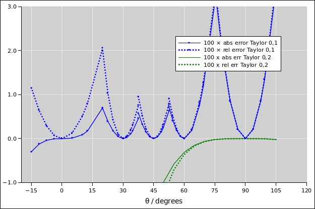
- This leaves us with a region from 10∘ to 25∘ that
requires some special attention. Options include the following:
For most purposes, the best option is to use the Taylor[1,3]
approximation anchored at zero. This requires a couple more
multiplications, but the result is accurate to better than 0.07%.
If you really want to minimize the number of multiplications, we can
start by noting that the Taylor[1] extrapolation coming up from zero
is better than the Taylor[0,1] extrapolation coming down from
30∘, so rather than using the closest anchor we use the 0∘
anchor all the way up to 20∘ and use the 30∘ anchor above
that. This has the advantage of minimizing the number of
multiplications. Disadvantages include having to remember an obscure
fact, namely the need to put the crossover at 20∘ rather than
halfway between the two anchors. The accuracy is better than 2.1%,
which is not great, but good enough for some applications. The error
is shown in figure 7.
There are many other options, but all the options I know of involve
either more work or less accuracy.
The spreadsheet that produces these figures is given by
reference 8.
Here are some additional facts that are needed in order to carry out
the calculations discussed here.
|
| |
1∘ | | = | | 17.4532925 milliradian | | | |
(5a)
|
|
| |
1 radian | | = | | 57.2957795∘ | | | |
(5b)
|
|
| |
sin(x) | | ≈ | | x | | for small x, measured in radians | |
(5c)
|
|
| |
cos(x) | | = | | sin(π/2 − x) | | for all x | |
(5d)
|
|
| | | ≈ | | 1 − x2/2 | | for small x, measured in radians | |
(5e)
|
|
Last but not least, we have the Pythagorean trig identity:
and the sum-of-angles formula:
|
sin(a + b) | | = | | sin(a)cos(b) + cos(a)sin(b) |
| (7)
|
If you can maintain even a vague memory of the form of equation 7, you can easily reconstruct the exact details. Use the
fact that it has to be symmetric under exchange of a and b (since
addition is commutative on the LHS). Also it has to behave correctly
when b=0 and when b=π/2.
If we assume b is small and use the small-angle approximations from
equation 5, then equation 7 reduces to the
second-order Taylor series approximation to sin(a+b).
|
sin(a + b) | | ≈ | | sin(a) + cos(a) b − sin(a) b2/2 | | for small b, measured in radians |
| (8)
|
If we drop the second-order term, we are left with the first-order
series, suitable for even smaller values of b:
|
sin(a + b) | | ≈ | | sin(a) + cos(a) b | | for smaller b, measured in radians |
| (9)
|
You can use the Taylor series to interpolate between the values given
in equation 4. Since every angle in the first quadrant
is at least somewhat near one of these values, you can find the sine
of any angle, to a good approximation, as shown in figure 6.
10 References
-
-
John Denker,
“Balancing Reaction Equations using Gaussian Elimination”
www.av8n.com/math/gauss-elim.htm
-
John Denker,
“Suggestions for Writing Good Software”
www.av8n.com/computer/htm/good-software.htm
-
Douglas Isbell, Mary Hardin, Joan Underwood
“MARS CLIMATE ORBITER TEAM FINDS LIKELY CAUSE OF LOSS”
http://mars.jpl.nasa.gov/msp98/news/mco990930.html
-
Google Calculator. Example: furlongs per fortnight,
converted to SI units:
http://www.google.com/search?q=1+furlong+per+fortnight+in+m/s
-
John Denker,
“Learning, Remembering, and Thinking”
www.av8n.com/math/thinking.htm
-
John Denker,
“Long Multiplication
www.av8n.com/math/long-multiplication.htm
-
John Denker,
“Long Division
www.av8n.com/math/long-division.htm
-
John Denker,
“spreadsheet for checking trig approximations
./trig-approx.xls