Introduction to Higher Math
John Denker
1 Preview
Let’s talk about “higher math” and its applications. For present
purposes, higher math means anything beyond arithmetic. The goal here
is not to teach you higher math, but merely to offer a few reasons why
you might want to go learn it, i.e. why you might find it interesting
and useful.
Let’s start with a simple yet practical example.
-
Suppose Mr. X lends a shovel to Mr. Y, and then
Mr. Y lends it to Mr. Z. When it comes time to return the
shovel, Z can return it directly to X, without having to go
through Y.
This rule applies to any X, Y, and Z.
This is the language of algebra, pure and simple.
In some official documents, one-letter names such as X, Y, and Z
are used in exactly this way, and indeed this is how the famous XYZ
Affair got its name; see reference 1. Other documents may use
somewhat longer names, such as John Doe and Richard Roe, which serve
exactly the same purpose. These are sometimes called dummy
names or placeholder names. A mathematician would call them
algebraic variables.
A great many important ideas are expressed using this sort of
language. In many cases it would be next to impossible to express
them any other way. It must be emphasized that this is already part
of the language, necessary for daily life, not limited to math and
science. However, studying math will give you a better understanding
of this language, and allow you to use it in more powerful ways.
-
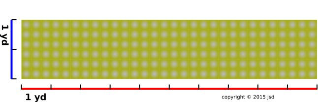
Here’s another simple yet very practical example that
uses mathematical ideas: Consider the hallway floor shown in figure 1. Using a yardstick, we find that the hallway is very nearly
rectangular, 10 yards long, and 2 yards wide.
We can express the length and width using simple equations:
|
| |
L | | = | | 10 yd | |
(1a)
|
|
| |
W | | = | | 2 yd | |
(1b)
|
|
where L represents the length, W represents the width, and yd
is an abbreviation for yard (or yards).
In the diagram, the length is shown in red and the width is shown in
blue. The black tick-marks show the length and width divided
into yards. We can write this as an equation:
|
| |
L / yd | | = | | 10 | |
(2a)
|
|
| |
W / yd | | = | | 2 | |
(2b)
|
|
Equation 2 is another way of formulating the same idea
as equation 1. Depending on circumstances, one formulation
or the other may be more convenient.
|
Note that in equation 2a the right-hand side of the
equation is a pure number, namely 10. The left-hand side of the
equation is also a pure number, because it is one length divided by
another length.
|
|
This stands in contrast to equation 1a, where
both sides of the equation are lengths, not pure numbers.
|
Equation 2 is one of those all-too-rare situations where
the language of English agrees with the language of algebra: The
length of the hallway can be divided into ten yards as surely as a
pizza can be divided into six slices. This is formalized by the
divide-by symbol on the left-hand side of equation 2a. We
can then count the subdivisions. This gives us the number on the
right-hand side.
This is an interesting lesson already, because it tells you that
mathematics is not just arithmetic. It is not limited to numbers. We
can write equations involving things like lengths (as in equation 1a) which are emphatically different from pure numbers (as in
equation 2a).
-
Now suppose we want to express the length in
terms of in feet (not yards). It’s the same length, just expressed in
different units. We could re-measure the length using a one-foot
ruler, but it is easier to figure it out mathematically. We can use
the following fact:
We can always multiply any expression by 1. This leaves the value
unchanged. (The rule about multiplying by 1 comes directly from the
laws of mathematics; it is a defining property of 1.) Let’s apply
this to equation 1a.
This trick of multiplying by 1 as a means of converting from one set
of units to another is called the factor label method. It is
very widely used. There are tons of pedagogical resources on the
topic. See also section 5.4.
This is an example of applied mathematics. This is also an example of
physics. That is, by combining some measurements and some
mathematics, we build a theoretical model that allows us to
ascertain something about the real world that we did not directly
measure. We know the length in feet, even though we didn’t measure it
directly using a one-foot ruler. You know it’s not pure mathematics,
because the result is not exact. It depends on various
approximations, notably the assumption that the floor is flat. If the
floor had lots of undulations, measuring it with a yardstick and
measuring it with a ruler might well give different lengths. For an
ordinary floor, however, the calculation in equation 4 is a
good-enough approximation for most purposes. See section 2.9 for more about the limitations of mathematics.
-
Things get even more interesting if we
want to know the area of the hallway floor.
There are ways of measuring the area of the floor directly – perhaps
by covering it with tiles of known area and counting the tiles – but
for a rectangular region it is quicker and more convenient to measure
the edges and multiply. For a rectangular region, the area is equal
to the length multiplied by the width. We can write this rule as an
equation:
Applying this rule to our hallway, we find:
|
A | | = | | L · W |
| | | = | | 10 yd · 2 yd |
| | | = | | 20 yd2
|
| (6)
|
where A denotes the area, and yd2 is pronounced “yard squared”
or equivalently “square yard”. It must be emphasized that when we
write a square yard as yd2 that does not mean two yards. It is
not a yard plus a yard. It is a yard times a yard. This is
part of the notation and terminology of mathematics: The small
superscript 2 means to multiply something by itself.
The approach used in equation 6 – combining
measurements with theory – is a lot less work than trying to measure
the area directly, even in this simple example. (In more complicated
situations, the advantage is even more dramatic.)
In equation 6, note the contrast:
|
Multiplying 10 by 2 to get 20 is just arithmetic. It’s just
numbers.
|
|
Multiplying a yard by a yard to get a square yard is higher
math.
|
A yard is not a number; it’s something else entirely. It is
proverbially improper to compare apples to oranges, and by the same
token it is improper to compare oranges to square yards. It’s also
improper to compare yards to square yards. If they were numbers you
could compare them, but they aren’t and you can’t. Yards and square
yards live in a high-dimensional abstract space of their own
... abstract yet very practical and very relevant to the real world.
-
Now suppose we want to express the area
in units of square feet. It’s the same area, just described in
different terms. We can use equation 3 to convert equation 6 using the same ideas as before, with a slight twist.
|
A | | = | | |
| | |
| | | = | | | 20 yd2 · | ⎛
⎜
⎜
⎝ | | ⎞
⎟
⎟
⎠ |
· | ⎛
⎜
⎜
⎝ | | ⎞
⎟
⎟
⎠ |
|
| | |
| | | = | | 180 ft2 |
| (7)
|
Notice that we had to multiply by 3ft/yd twice. That’s because we
started with yd2, which is a yard times a yard, and we need to
convert both factors. Even though one yard is equal to three feet, a
square yard is not equal to three square feet. In fact, a square yard
is equal to nine square feet, as you can see in figure 2. That’s a nontrivial fact.
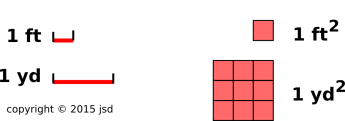 Figure 2
: Foot, Yard, Square Foot, and Square Yard
Note that the floor in figure 1 is tiled in one-foot squares.
You could determine the area directly by counting tiles, but it is
easier to measure the length and width and then ascertain the area by
multiplying.
Again our mathematical model is an excellent approximation to the real
world, but it is not exact. See section 2.9 and especially
example 2-1.
* Contents
2 Overview
2.1 Higher Math Topics
As mentioned in section 1, higher math means anything beyond
arithmetic. It includes the topics listed in table 1,
plus a tremendous amount of other stuff. Some of the applications are
mentioned in section 2.4 and elsewhere. We aren’t going to
explore all of higher math, just the easiest and most useful parts.
We assume you have never studied this in any depth before, or have
forgotten everything you learned about it.
| set theory | | logic | | probability |
| algebra | | calculus | |
| topology | | geometry | | trigonometry |
The most important thing you need to know is that math doesn’t have to
be weird or complicated. Like music or sports or anything else, if
you take it to extremes it can get very very complicated, but we
aren’t going to take it that far.
Generally speaking, math is a bag of tricks for reasoning about stuff
and solving problems. For a more detailed look at reasoning and
problem-solving in general, see reference 2 and reference 3.
2.2 Tools and Techniques – Preview
There are a lot of things that you need to learn that aren’t
officially listed as part of any ordinary course. These are
important, indeed more important than some of the things that are
listed.
| multi-step reasoning (section 8.2) | |
| higher reliability, stronger proof | |
| trusting certain tools | |
| avoiding certain booby traps | |
| skimming, reading, re-reading, and pondering a text (section 8.3) | |
| learning a new language | |
| generalization, symbolism, and abstraction | |
| imagination, creativity, artistry, and elegance | |
These things are related in various ways. For example, multi-step
reasoning demands high reliability, as discussed in section 8.2.
None of these things directly requires mathematics, or is restricted
to purely mathematical applications. For example, computer
programming requires all of those things, as surely as traditional
math does. See section 8.1 for more about this.
It must be emphasized that there is more to mathematics than right and
wrong. There is also elegance. Continuing down that road, there is
yet again more to applied math. There is not just right and
wrong, and not just elegance. There is also relevance and
practicality.
2.3 Higher Math is Not Arithmetic
It must be emphasized from the outset that higher math is dramatically
different from arithmetic. You don’t even need to be good at
arithmetic to do higher math.
Professional mathematicians do not sit around adding up long columns
of numbers. Really they don’t. They’ve got better things to do.
Higher math is an almost-completely different set of skills.
Basic arithmetic is devoid of the things that make math interesting,
including elegance and creativity. Arithmetic is relevant to higher
math in much the same way that arithmetic is relevant to cooking: It
is sometimes useful, but it’s not really the point.
Some mathematicians are really good at arithmetic, but some of them
aren’t. The ones in the latter group can certainly figure out
arithmetic problems, but they have to stop and think about it. Note
that mathematicians are allowed to use spreadsheets, just like
everybody else.
2.4 Applications Are Important: The Basket Analogy
Consider the analogy:
|
A wicker basket, by itself, it’s not good for much. You
can’t eat it. It doesn’t make a very good pillow, or a very good hat,
or very good underwear. If you’ve got nothing to store and nothing to
carry, the basket is not immediately practical. On the other hand, if
you have several important things to carry and somewhere to go, a
basket might be tremendously helpful.
|
|
Mathematical skills, by
themselves, are not good for much. However, when an application comes
along that calls for those skills, they can be tremendously helpful.
|
|
Sometimes you find something that looks like a basket but is
purely ornamental. Sometimes a weaver will make a basket just for
fun, or just to experiment, to see what’s possible and what’s not.
|
|
Sometimes people do math puzzles just for fun. Sometimes
mathematicians are motivated by pure esthetics, and sometimes by
curiosity, to see what’s possible and what’s not.
|
The so-called pure mathematicians pay little attention to
applications. According to legend, Euclid mocked a beginning student
who asked what geometry was good for. However, in my opinion, that’s
really bad pedagogy. Most of us are not pure mathematicians. I can
appreciate the artistry in an elegant mathematical proof, but that is
not the only thing I expect to get from mathematics.
Higher math is needed for:
- Physics. Even the simplest grade-school physics involves
notions of proportionality and conservation that are best expressed
in mathematical language. Introductory high-school physics is
completely dependent on the language of algebra. Anything beyond
that requires even more math, such as probability and calculus, not
just algebra.
Physicists tend to use all the math that is available, and more.
If necessary, they make it up as they go along. Isaac Newton
invented calculus for a reason: He needed it to solve physics
problems.
- Chemistry. Stoichiometry involves solving N linear
equations in N unknowns. A fairly simple pH calculation is
likely to turn into a cubic equation that needs to be solved.
- Engineering.
- Biology. Maybe a biologist could skate by without math 30
years ago, but not now. It’s all very quantitative and analytical
now. Even the art of medicine is gradually becoming quantitative
and analytical. See section 2.8.
- Computing. Nowadays computers are used in every branch of
science and technology, for entertainment, and for practically
everything else. Even a kindergarten teacher who doesn’t need to
know much in the way of physics, chemistry, engineering, or biology
has to deal with computers. The language of computing is based on
the language of algebra.
Computing (like higher math) is very different from arithmetic.
Computers are not just number crunchers. They also crunch text,
symbols, images, logic, and other abstractions.
2.5 Math is about Patterns and Relationships
A great deal of higher mathematics is devoted to patterns,
relationships, and generalizations ... finding them, creating them,
understanding them, et cetera. This can involve spatial patterns,
linguistic patterns, patterns in completely abstract systems, or
whatever. Sometimes mathematicians look for patterns in numbers, but
that’s not the only focus or even the main focus.
Some non-numerical examples are given in section 1 and
section 3. Meanwhile, some numerical examples are
given in section 4.
2.6 Math is a Language
Mathematics provides (among other things) a language that helps
us express ideas.
The language of algebra is already part of everyday conversations –
and the ideas of algebra are already part of everyday thought –
whether you realize it or not. It is not restricted to numbers. For
example, in example 1-1, the algebraic variables X, Y, and
Z refer to persons, not numbers.
Of course math is not just a language. Knowing the English
language does not make you a novelist; the primary requirement for
writing a novel is having something interesting to say. The language
just helps you say it. Math is primarily a bag of tools for reasoning
about stuff and solving problems. Mathematical language helps with
this, but it isn’t the main goal, and it isn’t the only tool.
Here’s another example: Consider the statement, “Conspiracy is
transitive”. That means if you conspire with X who conspires with
Y who conspires with Z, then all four of you are co-conspirators.
It is not necessary that each conspirator knows all of the others, or
knows all the activities of the conspiracy.
I mention this because normally people learn what “transitive”
means in the context of algebra, not crime.
- For example, if X is equal to Y and Y is equal to Z,
then we know X is equal to Z, because equality is transitive.
- Similarly, if X is greater than Y and Y is greater than
Z, then we know X is greater than Z, because the concept of
“greater than” is transitive.
The statement that “Conspiracy is transitive” is an example of
algebraic language and algebraic thinking in the real world. Algebra
changes the way you think.
Arithmetic is about numbers. Math is about patterns. For
example, when we say 9 is greater than 7, transitivity is not a
property of the number 9 or the number 7; transitivity is a property
of the “greater than” relationship.
2.7 Math is about Logic and Proofs
There is a tradition going back 2300 years that calls for studying
geometry in terms of proofs ... or vice versa. Euclid’s book is about
geometry in the same way that Orwell’s book is about animals,
i.e. hardly at all. Orwell’s animals are a backdrop and a pretext for
talking about politics. Euclid’s geometry is a backdrop and a pretext
for talking about proofs.
Some of the proofs that one encounters in high-school geometry are
elegant, intricate, and ingenious.
Beware that the mathematical approach has its limitations,
as discussed in section 2.9.
2.8 Math is Required for Science
Algebra and geometry are prerequisites for physics, biology,
chemistry, engineering, and computing.
Maybe 30 years ago, students who were interested in science but not
interested in mathematics might be advised to go into biology.
Nowadays, though, that would be very bad advice. The life sciences
(including medicine) have become intensely quantitative and
mathematical.
A while back I was out in the middle of the desert, helping some
graduate students who were studying Gila monsters. Whenever they
found one, they measured its height, width, length, tail volume, and
temperature. They recorded the location and environmental conditions.
For identification, they took a picture and implanted an electronic
RFID tag. Last but not least, they took a DNA sample.
All this went into a database. By analyzing the DNA, they were able
to construct lineages, showing who was related to whom. This step was
highly mathematical, involving reasoning about structures in an
abstract high-dimensional space.
On a more down-to-earth level, dealing with the location involved
geometry and algebra. They used GPS coordinates (which use one
ellipsoid) and then they needed to convert to map coordinates on an
out-of-date map (which used a different ellipsoid). If you don’t know
what an ellipsoid is, you are on the outside looking in. You can’t
even be part of the conversation.
2.9 Limitations of the Mathematical Approach
Although it is useful to learn the methods of mathematical proof (as
mentioned in section 2.7 and elsewhere), in practice the usual
“math textbook” style of deriving results has some serious
limitations.
- For one thing, although logical arguments work well for
convincing a scientist that you have the right answer, beware that
they don’t work very well at all for convincing the other 99.9% of
the population. Most people are not logical.
- If you want convenient and accurate techniques for measuring
geometrical shapes, you should use analytic geometry as discussed in
section 5.1, rather than the highly stylized
Euclidean constructions. We’ve made a lot of progress in the last
2000 years.
- If you are serious about learning proof techniques, you should
study modern notions of formal logic ... or modern computer
programming. The standards of proof in the computer industry are far
higher than the standards of proof in (say) Euclid’s Elements.
Euclid’s reasoning does not stand up to scrutiny under modern
standards; he assumes all sorts of things as he goes along, things
that should have been either proved or added to the list of
postulates. For some examples of this, see reference 4.
- When applying Euclidean deduction to the real world, you
need to have absolute confidence that the starting point – the set of
axioms – conforms to reality. The Euclidean axioms create a formal,
abstract world that is fine if all you care about is abstractions.
Alas, it is only tangentially relevant to real-world geometry.
The word “geometry” means, literally, measuring the earth, and the
study of geometry had its roots in surveying. The problem is, most of
Euclidean geometry assumes space has zero curvature, but real space is
curved. The actual surface of the earth is curved. When we include
the fourth dimension, spacetime is curved also. So we have a very
precise, formal, abstract system that does not describe the real
world. The best it can do is approximate the real world, in small
localized regions.
The sphericity of the earth was well known to Greek scholars long
before Euclid’s time.
Basic math results are sometimes considered exact, but science is
essentially never exact. We can see the distinction in the hallway in
example 1-2, example 1-3, example 1-4, and example 1-5. The rule
that says the area is equal to the length times the width only applies
to a rectangular region on a flat surface. However, a real-world
hallway is never exactly rectangular, and the surface of the earth is
not exactly flat. Furthermore, a real-world yardstick is never
exactly one yard long.
In reference 5, Einstein said “Insofar as the
propositions of mathematics refer to reality, they are not certain;
and insofar they are certain, they do not refer to reality”.
Religion offers certainty; science generally does not. Instead,
science teaches you how to survive and get things done in an uncertain
world.
-
This takes up where example 1-5 left off. Suppose we are buying tiles to cover
the floor of a hallway that is similar to figure 1 but not
identical: The floor is 30.2 feet long by 5.9 feet wide. The area is
less than 180 square feet, and each tile covers one square foot
... but we need more than 180 tiles. Calculating the area tells
us the number of tiles approximately but not exactly. The abstract
mathematical area is the answer to the wrong question. It’s almost
the right question, but not quite. In the real world, the objective
is not merely to cover the area, but rather to cover the area in a way
that looks nice. Covering the area using misshapen scraps of tile does
not look nice.
A better calculation is to round up to an integer number of tiles in
each direction, and then multiply. That gives us 6*31, which is 186
tiles. An even better calculation take into account the fact that
these tiles come in boxes of 20, so we have to round up again. We
have to buy 200 tiles, with the expectation that there will be some
leftovers.
Bottom line: Just because you have a theoretical model doesn’t mean it
is the correct theoretical model. When you calculate something, check
that you are calculating the right thing. Don’t grind out an exact
answer to the wrong question.
3 Some Simple Non-Numerical Examples
In this section, we present some examples that are
highly mathematical but not arithmetical.
3.1 Sudoku
Sudoku puzzles are logic puzzles, not arithmetic puzzles. They are
intensely mathematical, but not numerical. They do not require
multiplication or even addition.
Even though they are normally written using the digits {123456789},
the digits are not really representing numbers; you could equally well
write the puzzle in terms of the nine letters {abcdefghi}. More to
the point, you could write the puzzle in terms of letters that aren’t
in alphabetical order, such as the nine letters in the word
{sunflower}, as in the example below. You could also do it in terms
of nine abstract symbols that have no relationship to each other, such
as { ∇ ♒ ‡ ∧ © ≡
∞ ξ ☿ }.
Here is an example. The usual sudoku rules apply: each of the nine
symbols must appear once in each row, once in each column, and once in
each of the nine different 9×9 blocks. (The blocks are
indicated by the shading.) The symbols are the nine letters in the
word {sunflower}. Some of the symbols have been filled in, to help
you get started. The solution is given in
appendix 13.1.
3.2 Straight-Cut Origami
It must be emphasized that higher math includes a lot of things
besides algebra. Here’s an example that involves pure geometry, with
no algebra, and certainly no arithmetic. It’s a fold-and-cut puzzle:
Each student (or each 3-student team) gets a pair of
scissors plus a piece of paper with an arbitrary triangle drawn on
it. The mission, should you decide to accept it, is to cut out
the triangle using only a single straight cut. Hint: you may fold
the paper any way you like before cutting.
This puzzle is intensely mathematical – yet it involves no numbers,
no arithmetic, and no algebra. It is an interesting puzzle. It has
the advantage that you can pose it to people who don’t know any
physics, don’t know any algebra, and couldn’t multiply 44 by 5 without
a calculator.
Reference 6 is a news story that features this puzzle, and
offers some hope that the much-needed revolution in math education is
starting.
The puzzle comes from chapter 6 of reference 7. The book starts
out with an uncompromising manifesto of “art for art’s sake” ... but
as it goes along it mentions a few bits of math that started out
super-abstract but found important applications.
3.3 Functions
Consider the following six statements:
- If the fruit is a lemon then the color is yellow.
- If the fruit is a banana then the color is yellow.
- If the fruit is a cherry then the color is red.
- If the fruit is a McIntosh then the color is red.
- If the fruit is a Granny_Smith then the color is green.
- If the fruit is a lime then the color is green.
We can express the same information in a less verbose form, as shown
in table 3:
| fruit | | color |
| lemon | | yellow |
| banana | | yellow |
| cherry | | red |
| McIntosh | | red |
| Granny_Smith | | green |
| lime | | green |
Table 3: Color as a Function of Fruit
Grid 1 shows yet another way of expressing the same
information.
| | | yellow | | red | | green |
| lemon | | ✓ | | · | | · |
| banana | | ✓ | | · | | · |
| cherry | | · | | ✓ | | · |
| McIntosh | | · | | ✓ | | · |
| Granny_Smith | | · | | · | | ✓ |
| lime | | · | | · | | ✓ |
Grid 1: Color as a Function of Fruit
In this example, the grid representation is slightly less compact than
the tabular representation, but in other cases it may be more compact.
Furthermore, the grid representation is sometimes easier to interpret.
It is relatively easy to verify that there is only one checkmark per
row in grid 1. However, not all grids have this
property, as we can see in grid 2, where we
have lumped together both varieties of apple, and both kinds of
citrus. There are only four rows, but still six checkmarks.
| | | yellow | | red | | green |
| citrus | | ✓ | | · | | ✓ |
| banana | | ✓ | | · | | · |
| cherry | | · | | ✓ | | · |
| apple | | · | | ✓ | | ✓ |
As a point of terminology, in grid 1 we say that the
color is a function of the type of fruit. The defining
property of a function is that there is only one checkmark per row.
This stands in contrast to grid 2, where color
is not a function of the category of fruit. There is a
relationship between color and the category of fruit, but this
relationship does not qualify as a function.
Very commonly non-experts say “function” even when the relationship
is not a function, but this is a mistake.
On the other hand, given a well-behaved non-function, it is usually
possible to create a function, using the idea of sets. Table 4 shows how this works when applied to our
example.
| fruit | | set of colors |
| citrus | | {yellow, green} |
| banana | | {yellow} |
| cherry | | {red} |
| apple | | {red, green} |
Table 4: Set of Colors as a Function of Fruit
Note that color itself is still not a function of the category of
fruit. Instead it is a set of colors that exists as a function
of the category of fruit in this example.
There is a subtle distinction between “color” and “set of colors”
– but the distinction is important. The idea of “set” is
completely abstract, but it’s not very complicated.
4 Some Simple Numerical Examples
In this section, the algebraic variables represent numbers.
4.1 The Meaning of Equality versus Recipe
Consider simple arithmetic problems such as the following:
| Fill in the blank: |
| 7 + 3 | | = | | ____
|
| (8)
|
|
|
| Fill in the blank: |
| ____ | | = | | 7 + 3
|
| (9)
|
|
Nowadays students are asked to solve problems like this in
kindergarten. Note that there are two ways of reading such a problem:
- Carry out the operations on the left-hand side (LHS) of of
equation 8, and use that as a recipe to find a value for
the RHS.
- Find a value for “____” that makes the equation true.
These two readings are significantly different.
- The “recipe” in equation 8 is strictly
left-to-right. It would be nonsense to use the RHS as a recipe for
computing the LHS.
Meanwhile, equation 9 is strictly right-to-left.
- Any reasonable notion of equality is symmetrical. For example,
if 1 yd = 3 ft then 3 ft = 1 yd. You can read the
equation either way, left-to-right or right-to-left. The “find a
value” reading is symmetrical, and works just fine for a very wide
class of equations, including equation 10 in addition to
equation 8 and equation 9. (In contrast, the
“recipe” interpretation fails for equation 10.)
| Fill in the blank: |
| 7 + ____ | | = | | 10
|
| (10)
|
The existence of problems such as equation 10 is a Big Deal
conceptually and pedagogically. Any students who latch onto the idea
that every equation is a recipe (as in equation 8) will
have to unlearn that before they can cope with equation 10.
Unlearning is always hard.
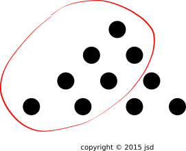
Figure 3 shows one way of solving equation 10,
namely a graphical method. Start with a group of ten things. Draw a
loop around seven of them. The number remaining outside the loop is a
solution to equation 10. This can be seen from the fact that
the number inside plus the number outside adds up to 10.
Another way to solve the problem is by counting on your fingers,
performing a calculation essentially equivalent to figure 3.
Yet another way to solve the problem is by using an addition table,
such as the one shown in table 5. Find the 7th column, and
run down that column until you find a 10. The corresponding
row-number is the solution to the problem.
There also exists a purely mathematical recipe for solving problems of
this kind – a recipe called subtraction – but equation 10 does not explicitly depend on subtraction. We do not need any
minus signs in order to write equation 10. In fact, the idea
behind equation 10 can be used to define what we mean by
subtraction.
There’s a name for what we’re doing here: It’s called algebra.
Equation 10 is not very fancy algebra, but it is definitely
algebra. Note the contrast:
|
10 − 7 = ____ is not algebra. It’s just arithmetic.
You’re doing subtraction because you were told to do subtraction.
|
|
7
+ ____ = 10 is algebra. You might solve it by doing subtraction,
but the equation doesn’t tell you to do that. You have to apply some
mathematical reasoning to change the given equation into a subtraction
problem.
|
The distinction between 10 − 7 = ____ and 7 + ____ = 10 is
is like crossing from Nogales, Arizona to Nogales, Sonora. You aren’t
very far from the border, but you’re definitely in a different
country. The equation 7 + ____ = 10 is definitely on the algebra
side of the border.
4.2 Two Unknowns
Let’s consider some much fancier than equation 10, namely
equation 11. Equations like this show up in school, sometimes
even at kindergarten level nowadays:
| Fill in both blanks: |
| ____ + ____ | | = | | 10
|
| (11)
|
This equation has the remarkable property that it has
more than one solution. For example, 3 + 7 = 10 and
also 6 + 4 = 10.
One way of solving this problem uses the method outlined in figure 3. Start with a group of ten things, then draw a
circle around any number of them, any number from zero on up, any
number from zero to ten inclusive. The number inside and the number
outside can be used to fill in the blanks in equation 11.
Another way of solving this problem is to use an addition table, such
as table 5. Look through the table until you find a 10
somewhere. Then read off the column number and the row number.
Some people go bonkers when they see a question of this kind.
Sometimes for political or cultural reasons they think the most
important thing is for every student to get the same answer, and it
horrifies them to think that different students might come up with
different yet fully-correct answers.
In kindergarten, the students are asked to find some solution to
the problem, i.e. some way of filling in the blanks. In
contrast, a mathematician looks at equation 11 and wants to
find all solutions.
- If we restrict attention to non-negative integers, we can find
all the solutions with the help of table 5. We can easily
find every 10 in the table. They all like along a diagonal line.
There are exactly 11 of them. In other words, there are 11
possible solutions.
- If we allow fractions, such as 6½ + 3½ = 10, there are
infinitely many ways of solving the equation.
- If we allow negative numbers, such as −3 + 13 = 10, there are
infinitely many ways of solving the equation.
It is quite remarkable that equation 10 has exactly one
solution, while equation 11 can have infinitely many
solutions. The two equations look somewhat different, but they don’t
look infinitely different.
We are definitely doing higher math now. Basic arithmetic does not
produce infinities, and cannot deal with infinities. Arithmetic deals
with numbers, whereas infinity is not a number. Higher math deals
with all sorts of things that aren’t numbers.
We can make equation 11 look fancier by giving names
to the unknowns.
| Find some x and y to solve the equation: |
|
| |
x + y | | = | | 10 | | |
(12a)
|
|
| |
x | | = | | ____ | | |
(12b)
|
|
| |
y | | = | | ____ | | |
(12c)
|
|
That may look fancier than equation 11, but it has exactly the
same meaning.
Note that in a system of equations like this, the x in equation 12a must have the same value as the x in equation 12b. By the same token, the y in equation 12a
must have the same value as the y in equation 12c. We get
to choose a value for x, but whatever we choose has to be
consistent across the whole problem, across the whole system of
equations. See section 4.15.
We can apply that idea in a useful way in equation 13.
This is equivalent to equation 11 with the added requirement
that the same number must be used to fill in both blanks.
| Find some x to solve the equation: |
|
| |
x + x | | = | | 10 | | |
(13a)
|
|
| |
x | | = | | ____ | | |
(13b)
|
|
In equation 13 and elsewhere, the rule is: In any given
system of equations, every time x appears, it has to have the same
value. In equation 12, x can be different from y
... but x cannot be different from x.
Note that equation 13 has only one solution, whereas
equation 12 has many solutions.
4.3 Addition Table
| 0 | | 1 | | 2 | | 3 | | 4 | | 5 | | 6 | | 7 | | 8 | | 9 | | 10 | | |
| 1 | | 2 | | 3 | | 4 | | 5 | | 6 | | 7 | | 8 | | 9 | | 10 | | 11 | | |
| 2 | | 3 | | 4 | | 5 | | 6 | | 7 | | 8 | | 9 | | 10 | | 11 | | 12 | | |
| 3 | | 4 | | 5 | | 6 | | 7 | | 8 | | 9 | | 10 | | 11 | | 12 | | 13 | | |
| 4 | | 5 | | 6 | | 7 | | 8 | | 9 | | 10 | | 11 | | 12 | | 13 | | 14 | | |
| 5 | | 6 | | 7 | | 8 | | 9 | | 10 | | 11 | | 12 | | 13 | | 14 | | 15 | | |
| 6 | | 7 | | 8 | | 9 | | 10 | | 11 | | 12 | | 13 | | 14 | | 15 | | 16 | | |
| 7 | | 8 | | 9 | | 10 | | 11 | | 12 | | 13 | | 14 | | 15 | | 16 | | 17 | | |
| 8 | | 9 | | 10 | | 11 | | 12 | | 13 | | 14 | | 15 | | 16 | | 17 | | 18 | | |
| 9 | | 10 | | 11 | | 12 | | 13 | | 14 | | 15 | | 16 | | 17 | | 18 | | 19 | | |
| 10 | | 11 | | 12 | | 13 | | 14 | | 15 | | 16 | | 17 | | 18 | | 19 | | 20 | | |
The addition table has some interesting properties.
- The table can used as follows. For example, the cell at the
intersection of row #2 with column #3 contains the value 5, which
is the sum of 2 and 3. Similarly the cell at the intersection of row
#4 and column #6 contains the value 10, which is the sum of 4 and
6.
- The table can be used in other ways as well. For example, to
solve the equation 7 + ____ = 10, look in row #7 to find the
number 10. The corresponding column number is the solution to the
problem. In other words, if you use it backwards, the addition table
can be used to perform subtraction.
- You can construct the addition table without actually doing any
addition. You can construct any row just by counting: 4, 5, 6 et
cetera. Ditto for any column.
- The table has a mirror symmetry. The axis of symmetry is the
main diagonal, starting from 0 and running toward the lower right.
If you flip or reflect the table about that axis, all the numbers are
unchanged. This symmetry corresponds to the fact that addition is
commutative.
- Here’s an even stronger symmetry: If you find all the fours in
the table, they fall along a diagonal. Ditto for all the fives. In
table 5, all the fives are colored red, to highlight this
pattern.
Conversely, if you pick any diagonal running parallel to the
direction from lower-left to upper-right, all the numbers along that
diagonal are the same.
- A simplified version of the same idea says that starting
from any given cell, moving downwards one step gives the
same result as moving rightward one step.
We can express this rule as an algebraic formula:
| For any row C and any column R, |
| (R+1) + C | | = | | R + (C+1) |
|
| (14)
|
Mathematicians use this property as part of the formal definition of
what we mean by addition. We don’t need to delve into the details;
the interesting point is that there actually is a formal definition
of “integer” and a formal definition of “addition”.
- The top row of the table serves as a header, labeling the
various columns ... but it is also part of the body of the table, in
the sense that it gives the result of adding zero plus something.
Similarly, the leftmost column serves to label the various rows
... but it is also part of the body of the table, giving the result
of adding something plus zero. (In contrast, most other tables
require row labels and/or column labels that are separate from the
body of the table, as you can see in grid 1 for
example.)
Note the contrast:
|
Constructing the addition table is just arithmetic. Using
the table to perform addition is just arithmetic.
|
|
Looking for
symmetries and patterns in the table is higher math.
|
4.4 Multiplication Table
| 1 | | 2 | | 3 | | 4 | | 5 | | 6 | | 7 | | 8 | | 9 | | 10 | | | |
| 2 | | 4 | | 6 | | 8 | | 10 | | 12 | | 14 | | 16 | | 18 | | 20 | | | |
| 3 | | 6 | | 9 | | 12 | | 15 | | 18 | | 21 | | 24 | | 27 | | 30 | | | |
| 4 | | 8 | | 12 | | 16 | | 20 | | 24 | | 28 | | 32 | | 36 | | 40 | | | |
| 5 | | 10 | | 15 | | 20 | | 25 | | 30 | | 35 | | 40 | | 45 | | 50 | | | |
| 6 | | 12 | | 18 | | 24 | | 30 | | 36 | | 42 | | 48 | | 54 | | 60 | | | |
| 7 | | 14 | | 21 | | 28 | | 35 | | 42 | | 49 | | 56 | | 63 | | 70 | | | |
| 8 | | 16 | | 24 | | 32 | | 40 | | 48 | | 56 | | 64 | | 72 | | 80 | | | |
| 9 | | 18 | | 27 | | 36 | | 45 | | 54 | | 63 | | 72 | | 81 | | 90 | | | |
| 10 | | 20 | | 30 | | 40 | | 50 | | 60 | | 70 | | 80 | | 90 | | 100 | | | |
The multiplicationtable has some interesting properties.
- The table can used as follows. For example, the cell at the
intersection of row #2 with column #3 contains the value 6, which
is the product of 2 and 3. Similarly the cell at the intersection of
row #4 and column #6 contains the value 24, which is the product of
4 and 6.
- The table can be used in other ways as well. For example, to
solve the equation 3 × ____ = 12, look in row #3 to find
the number 12. The corresponding column number is the solution to
the problem. In other words, if you use it backwards, the
multiplication table can be used to perform division.
If you try to solve the equation 3 × ____ = 16, you find
there is no solution. That tells us that 16 is not divisible by 3.
(In this context, “not divisible” means “not evenly divisible”.)
- You can construct the multiplication table without actually
doing any addition. You can construct any row just by adding.
For example, the second row can be constructed by counting
by twos, and the third row can be constructed by counting
by threes. The same is true of any column.
We can express this rule as an algebraic formula:
| For any row C and any column R, |
| R × (C+1) | | = | | R × C + R |
|
| (15)
|
Mathematicians use this property as part of the formal definition of
what we mean by multiplication.
- The table has a mirror symmetry. The axis of symmetry is the
main diagonal, starting from 1 and running toward the lower right.
If you flip or reflect the table about that axis, all the numbers are
unchanged. This symmetry corresponds to the fact that multiplication
is commutative.
- The top row of the table serves as a header, labeling the
various columns ... but it is also part of the body of the table, in
the sense that it gives the result of multiplying one times
something. Similarly, the leftmost column serves to label the
various rows ... but it is also part of the body of the table, giving
the result of multiplying something times one.
- The numbers on the main diagonal
are the square numbers: 12=1,
22=4, 32=9, 42=16, et cetera.
4.5 Relationships and Operators
The language of algebra can be used in many ways. Sometimes it is
used to set up an equation to be solved. That’s the first thing some
people think of when you mention algebra, but it’s by no means the
only thing that algebra is good for.
Consider the contrast:
|
Setting up an equation to be
solved.
|
|
Asserting a relationship.
|
|
In statement 16, the goal is to find a numerical
value for x. The equation tells us about a particular number x.
|
|
In statement 17, it is not necessary, desirable, or
possible to solve for x or y.
|
|
|
| |
Find a value for x such that | | | |
(16a)
|
|
| |
2x − 7 = 1 | | | |
(16b)
|
|
|
|
|
| |
For all real numbers x and y, | | | |
(17a)
|
|
| |
(x + y) = (y + x) | | | |
(17b)
|
|
|
Statement 17 is not restricted to any particular
numbers. It is a powerful generalization. In one sense, it is a
general statement about all real numbers. In an even grander
sense it is a general statement about the addition operator itself: It
says that addition is commutative (when applied to real numbers).
Let’s be clear: The plus sign in equation 17b represents the addition operator.
Addition is quite an abstract thing. It’s definitely not a number.
Algebra gives us a language that allows us to say useful things about
addition itself. Similarly it allows us to talk about other highly
abstract things.
Suppose you see just the “equation” part of an algebraic statement
by itself, such as equation 16b or equation 17b. The meaning of such a thing by itself
would not be clear. You need the full statement. Note the contrast:
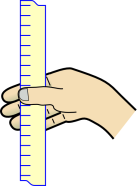
4.6 Reaction Time
You can measure human reaction time using little more than a
yardstick. People who have never seen a reaction-time measurement
tend to be very surprised at how long reaction times really are.
For details, see reference 8.
4.7 Brownies
Suppose you want to make brownies to feed 15 people. All the brownies
must all be rectangular, with the same size and shape, one per person.
For esthetic reasons, we want the aspect ratio to be no bigger than
1.5 to 1. That is, the length must be no more than 1.5 times the
width. The brownie pan is square.
You can’t do it with exactly 15 brownies. You could make 3 rows of 5
but that doesn’t satisfy the aspect-ratio requirement.
You can however make 16 brownies and have one left over. That’s
four rows of four.
The same solution works for 16 people, with nothing left over. In
fact, the 4×4 solution is optimal for 13, 14, 15, or 16 people.
For 17 people, we need to find a different solution. 17 is a prime
number, so that’s definitely not going to work. 18 can be factored as
3 rows of 6 or 2 rows of 9, but neither of those satisfies the
aspect-ratio requirement.
19 is a prime number, so that’s not going to work. 20 works, namely 4
rows of 5. For 17 people, that leaves three left over. In fact the
4×5 solution is optimal for 17, 18, 19, or 20 people.
The 4×6 solution is optimal for 21, 22, 23, or 24 people.
The 5×5 solution is optimal for 25 people.
For present purposes, we define optimal to mean satisfying the
requirements with minimal leftovers.
The question arises, how do we know that these are the only solutions?
Well, we could do it by brute force, just multiplying together all
pairs of numbers and seeing what works. However, mathematics gives us
an easier way. We can appeal to the unique-factorization theorem. It
says that any given integer can be factored using prime numbers in
exactly one way (except for trivial re-ordering of the factors).
- For example, 5 is a prime number, and 25 can be factored as
5×5, so we know that 5×5 and 25×1 are absolutely
the only possibilities.
- Similarly, 24 can be factored as 2×2×2×3. We
can group the factors as 3×8, 6×4, 12×2, or
24×1. We know there are no other possibilities. Of these,
only 6×4 satisfies the aspect-ratio requirement.
The goals and requirements can be expressed in mathematical language.
For N people we have:
|
A × B | | ≥ | | N |
| A ÷ B | | ≥ | | 2/3 |
| A ÷ B | | ≤ | | 3/2 |
| A × B as small as possible | |
| (18)
|
4.8 Economical Car
Suppose you are shopping for a car. The question arises, does it make
sense economically to get a hybrid car, or to get the corresponding
non-hybrid car. The answer depends on how the car is to be used, so
let’s consider two different scenarios.
First scenario: used as taxi, 25,000 miles per year, all city driving.
| | Car #1 | | Car #2 | | |
| | Camry LE | | Camry Hybrid LE | | units |
| | | | | | |
| purchase price | 24000.00 | | 28000.00 | | $ |
| | | | | | |
| delta | | 4000.00 | | | |
| | | | | | |
| hwy mileage | 35.00 | | 39.00 | | mpg |
| city mileage | 25.00 | | 43.00 | | |
| | | | | | |
| | | | | | |
| travel | | 25000.00 | | | miles per year |
| fraction on highway | | 0.00 | | | dimensionless |
| | | | | | |
| gas unit cost | | 3.00 | | | $ per gallon |
| | | | | | |
| gas volume | 1000.00 | | 581.40 | | gallons per year |
| gas cost | 3000.00 | | 1744.19 | | $ per year |
| | | | | | |
| delta | | -1255.81 | | | $ per year |
| | | | | | |
| | | | | | |
| payback time | | 3.19 | | | years |
Second scenario: Same two cars, retired person, much less driving,
mostly on the highway.
| | Car #1 | | Car #2 | | |
| | Camry LE | | Camry Hybrid LE | | units |
| | | | | | |
| purchase price | 24000.00 | | 28000.00 | | $ |
| | | | | | |
| delta | | 4000.00 | | | |
| | | | | | |
| hwy mileage | 35.00 | | 39.00 | | mpg |
| city mileage | 25.00 | | 43.00 | | |
| | | | | | |
| | | | | | |
| travel | | 5000.00 | | | miles per year |
| fraction on highway | | 0.75 | | | dimensionless |
| | | | | | |
| gas unit cost | | 3.00 | | | $ per gallon |
| | | | | | |
| gas volume | 157.14 | | 125.22 | | gallons per year |
| gas cost | 471.43 | | 375.67 | | $ per year |
| | | | | | |
| delta | | -95.76 | | | $ per year |
| | | | | | |
| | | | | | |
| payback time | | 41.77 | | | years |
We see that in the first scenario, the hybrid is a good deal. The
more expensive car quickly pays for itself via improved fuel economy.
In the second scenario, the more expensive car does not pay for
itself.
This is a simplified analysis. It is a reasonable first
approximation, suitable for cases where the conclusions are clear-cut.
For more marginal situations, a more sophisticated calculation is
required, taking into account interest rates, inflation, et cetera.
One way to formalize this is to calculate the Net Present Value.
Remember, arithmetic is about numbers, whereas higher math is about
patterns. So far we have only done a bunch of arithmetic.
This example begins to touch on higher math if you decide that doing
the arithmetic by hand is too laborious and too error prone, so you do
it using a spreadsheet instead. The language for programming a
spreadsheet is essentially the language of algebra.
This example becomes truly higher math when you try to understand
the trends:
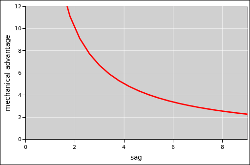
- How does the payback time depend on the capital cost, i.e. the
purchase price of the two cars? It turns out that it is proportional
to the difference in price.
- How does the payback time depend on the gas mileage of the two
cars? It turns out that it is inversely proportional to the
difference in mileage, for any given style of driving.
- How does the payback time depend on the unit cost of gasoline?
It turns out that it is inversely proportional.
- How does the payback time depend on the style of driving,
i.e. city versus highway? This is tricky; the inverse payback time is
a linear function of the percentage of city driving, but it’s not
purely proportional.
The spreadsheet used to do these calculations is given in reference 9.
4.9 Squares and Square Roots
Let’s review some basic facts:
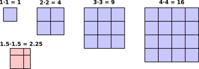
-
If the EdgeLength of a square is 2 inches, then the Area is 4
square inches. You can verify this by counting the little sub-squares
in figure 5.
-
If the EdgeLength of a square is 3 inches, then the
Area is 9 square inches.
-
The general rule for finding the Area of a square is
to multiply the EdgeLength times itself, in accordance with equation 19. This is a lot quicker and more reliable than counting
sub-squares, especially when the area is large.
|
Area | | = | | EdgeLength · EdgeLength
|
| (19)
|
-
The same procedure works even if the EdgeLength is not an
integer, i.e. not a whole number. For example, if the EdgeLength is
1.5 inches then the area is 2.25 square inches.
- The easiest way to obtain this result is by multiplying, in
accordance with equation 19.
- You can also verify this result by counting the full
sub-square, the two halves of a sub-square, and the quarter
of a sub-square within the light red square in figure 5.
-
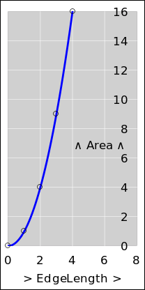
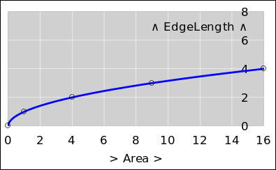
We can also use graphs to show the relationship between
EdgeLength and Area, as in figure 6 or equivalently
figure 7.
It must be emphasized that these two figures convey exactly the same
information. If you prefer one over the other, that is mostly a
matter of personal taste. There are four possibilities, all of which
work equally well:
- You can use figure 6 to convert from Area to EdgeLength
or vice versa.
- You can equally well use figure 7 to convert from
Area to EdgeLength or vice versa.
There is a lot more that can be done with such graphs, as discussed in
section 6.5.
-
Consider the contrast:
|
Sometimes we know the EdgeLength and want to calculate the
Area.
|
|
Sometimes we know the Area and want to calculate the
EdgeLength.
|
|
We say 9 the square of 3. This comes up so often that
there is a special notation for it, using a superscript 2. The
expression 32 is usually pronounced “three squared” and the
expression 52 is usually pronounced “five squared”.
|
| |
9 | | = | | 32 | | (exactly) | |
(20a)
|
|
| |
16 | | = | | 42 | | (exactly) | |
(20b)
|
|
| |
2 | | = | | 1.4142 | | (very nearly) | |
(20c)
|
|
|
|
We say 3 is the square root of 9.
This comes up so often that there is a standard abbreviation for it
(sqrt), and even a standard symbol (√). The expression
√3 is pronounced “square root of three”.
|
| |
3 | | = | | sqrt(9) | | (exactly)
| |
(21a)
|
|
| |
4 | | = | | √(16) | | (exactly)
| |
(21b)
|
|
| |
1.414 | | = | | √(2) | | (very nearly)
| |
(21c)
|
|
|
|
You can calculate the square of any number by direct
multiplication, in accordance with equation 19. You can also
read off the answer from a graph such as figure 6 or
figure 7.
|
|
There are procedures for calculating the
square root of any number. Details can be found in reference 10. For now, you can just read off the answer from a graph
such as figure 6 or figure 7. Also, any
spreadsheet program and virtually any pocket calculator will calculate
square roots for you. Look for the calculator key labeled with the
√ symbol.
|
-
The EdgeLength verus Area relationship is the
inverse of the Area versus EdgeLength relationship (and vice
versa). In other words, if we restrict attention to non-negative
numbers, the “square” relationship is the inverse of the
“square root” relationship.
This is important, because it gives you a way to check your
work. If you are not sure that equation 21c is correct, you
can check it by calculating the square of 1.414 by direct
multiplication, and comparing with equation 20c. We can
express the general rule using the language of algebra: For
any non-negative number X
4.10 Some Generalizations
-
In general, the Area of a rectangle is equal to
the Length of edge X multiplied by the Length of side Y (where
X and Y are perpendicular). This should be obvious from basic
notions of counting squares. If you remember the formula for a
rectangle, you don’t need to separately remember the formula for a
square, because a square is just a special kind of rectangle, namely
the kind where X=Y.
I could have mentioned this in section 4.9 but I didn’t,
because it was more than we needed to know at the time.
-
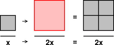
Let’s talk about scaling. You may be
familiar with the term, perhaps in connection with scaling up a
recipe, if you want to make twice as many cookies.
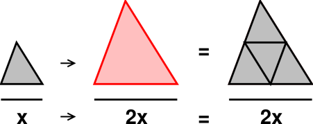
The idea expressed in figure 5 and figure 8 is
not limited to square-shaped figures.
The same sort of thing happens with triangles, as shown in figure 9. When the edge of the triangle grows by a factor of two,
the area of the triangle grows by a factor of two squared, i.e. 22,
i.e. 4.
The general idea here is that the triangle is a two-dimensional
figure, while the edge is one-dimensional. When we increase the edge
by a factor of 2, we increase both the horizontal and vertical
size of the triangle by a factor of 2, so the area goes up by two
factors of 2.
If we increase the edge by a factor of 3, then the area goes up by a
factor of 32 i.e. three squared i.e. 3×3 i.e. 9.
The same logic applies to any two-dimensional figure, not just
triangles and squares. This is called scaling. For more on
this, see reference 11.
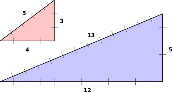
4.11 Diagonal Distances
If you move 4 units horizontally and 3 units vertically, you wind up 5
units from where you started, as the crow flies. Similarly, if you
move 12 units horizontally and 5 units vertically, you wind up 13 units
from where you started, as the crow flies. This is shown in
figure 10.
Now suppose you move B units straight horizontally and A units
straight vertically, and you find yourself C units in a straight
line from where you started. The general rule (subject to mild
restrictions) is that these distances obey the equation:
|
| |
A·A + B·B | | = | | C·C | |
(23a)
|
|
| |
A2 + B2 | | = | | C2 | |
(23b)
|
|
Equation 23b is entirely equivalent to
equation 23a. In accordance with standard notation, A2
is pronounced “A squared” and means to multiply A by itself.
Equation 23 is a famous result, known as the Pythagorean
theorem. It has been known for more than 2500 years. It tells us
something important about the structure of the universe. It didn’t
have to be that way. In particular, it only works for straight lines
in a flat plane; if you measure great-circle distances on the surface
of a sphere, the distances do not uphold equation 23 (unless
the triangles are very small). Also, equation 23 does not
apply to every triangle in the world; it only applies to right
triangles, i.e. triangles where the A-side is perpendicular to the
B-side.
4.12 Application: Cutting an Octagon from a Square
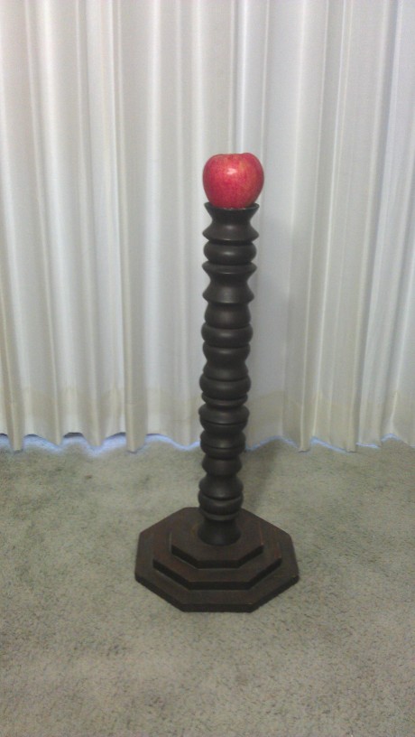
Here is a completely non-imaginary application.
In high-school wood-shop class I made an elaborately-carved
two-foot-tall candlestick, as shown in figure 11.
It needed a base. I decided that a multi-tiered octagonal base
would look nice. Starting from a square piece of wood, you can make
an octagon by cutting off the corners, but the question is, how much
to cut? You could solve the problem using purely mechanical
geometrical means, but it is just as easy to solve it using algebra.
So, suppose we have a square piece of wood, one foot on a side. We
wish to make an octagon by cutting off the corners. Suppose we cut
off a certain amount from each corner, as shown in figure 12.
We don’t yet know the correct amount, but that’s OK, so long as we
know x at the end. That’s one of the things (but not the only
thing) that algebra is good for: If you don’t know exactly what
something is, call it x and move on.
For the octagon, it is a simple matter to solve for x. Algebra
gives us a systematic way of finding a value for x that will make
all sides of the octagon equal in length.
After drawing the diagram, the next step is to write some algebraic
equations that involve x. We then solve the equations to find the
desired numerical value.
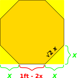 Figure 12
: Cutting An Octagon Out of a Square
We now use two separate lines of reasoning to calculate two different
sides in terms of x:
- By subtraction, we know that the length of the horizontal side
of the octagon is
|
length[horizontal] | | = | | 1 ft − 2x
|
| (24)
|
- Using the Pythagorean theorem, we know length of the sloping
side is:
Since we want it to be a regular octagon, the two “different”
sides are different only as to orientation; they are equal in length.
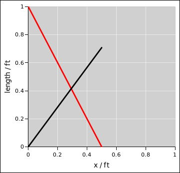
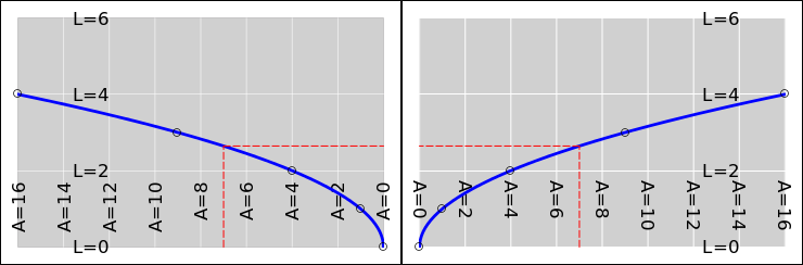
We can visualize what is going on by making a graph, although this is
not necessary. The length of the horizontal side (as given by
equation 24) is shown in red, while the length of the
sloping side (as given by equation 25) is shown in black.
The requirement that the sides must have equal length is represented
by the intersection of the two lines. By reading the chart you can
see that the x-value must be slightly less than 0.3 and the
corresponding length-value must be slightly more than 0.4.
Whether or not we have made a graph, we can express the requirement
that the sides of the octagon are equal by combining equation 24 and equation 25 in to a single algebraic
equation:
|
length of | | | | length of |
| sloping side | | = | | horizontal side |
| | = | | 1 ft − 2x
|
| (26)
|
We can solve it using a sequence of algebraic steps. At each step, we
show the rationale and method for obtaining the next equation.
|
| | Rationale (R) and Method (M) | | Equation |
| | |
| M: Restate equation 26. | |
|
| |
| | | = | 1 ft − 2x
| |
(27a)
|
| R: We want all terms involving x | |
| to be on one side. | |
| M: Add 2x to both sides. | |
|
| |
| | | = | 1 ft
| |
(27b)
|
| R: We want “something” times x. | |
| M: Distributive law. | |
|
| |
| | | = | 1 ft
| |
(27c)
|
| R: We want x by itself. | |
| M: Divide both sides by 2+√2. | |
|
| |
| | x | = | | |
(27d)
|
| Convert to decimal numeral. | |
|
| |
| | x | = | 0.2929 ft
| |
(27e)
|
|
Last but not least, we should always check our work. The two sides of
the octagon have the following lengths:
|
| |
horizontal side | | = | | 1 ft − 2x | = | 0.4142 ft
| |
(28a)
|
|
| |
sloping side | | = | | | = | 0.4142 ft
| |
(28b)
|
|
We see that the two sides have the same length, as they should, even
though they were calculated in very different ways. We can verify
after marking and before cutting that the sides have the correct
length.
The algebraic technique we have used here is called “solving two
linear equations in two unknowns” – but if that doesn’t mean
anything to you, don’t worry about it.
4.13 Graphs, Tables, and Functions
Another big part of algebra is the idea of a function.
Unlike variables, which are already part of everyday language and
everyday thought, the idea of a function is something that you may
have to think about before you fully understand it.
The basic idea is that a function is a recipe. It is a machine that
takes certain things as inputs, performs some manipulations, and
produces something else as the output.
For details on this, see section 6.
4.14 Example: Medicine Schedule and Dosage
Coming soon.
4.15 Key Concept: Pick Consistent Values
This continues the discussion of consistency from section 4.2. Consider the following:
|
| |
5·(1001) | | = | | 5005 | | | |
(29a)
|
|
| |
5·(1002) | | = | | 5010 | | | |
(29b)
|
|
| |
5·(1003) | | = | | 5010 | | | |
(29c)
|
|
| |
5·(1000 + x) | | = | | 5000 + 5·x | | (for all x) | |
(29d)
|
|
Equation 29d uses the language of algebra to summarize the
pattern we see in the previous lines. It is a powerful
generalization. If you have 1000 plus something, and you multiply the
whole thing by five, you multiply the 1000 by five and multiply the
other thing by five. This is an example of what we call the
distributive law.
It is crucial to choose the same value of x on both sides of
the equation; otherwise you get nonsense. This is one of the most
fundamental rules of algebra. It is so fundamental that it is often
left unstated, but don’t let that fool you.
Don’t change horses in mid-stream.
Don’t change the meaning of x in mid-calculation.
|
|
|
|
So long as you choose the same value of x on both sides of the
equation, you can use any x-value you like. Equation 29d
applies for all x. It applies for each and every x that you care
to choose.
You are allowed to have more than one horse, so long as you keep track
of which is which.
5 More about Algebra
5.1 Algebra Enriches Geometry
The roots of geometry can be traced back more than 3000 years. The
roots of algebra can be traced back even farther. For most of that
time, until about 300 years ago, they were separate. However, algebra
plus geometry together is more interesting than either of them
separately. Basic geometry plus algebra gives you trigonometry.
More generally, geometry plus algebra gives you the even larger field
known as analytic geometry.
-
-
Here’s an example of a real-world
problem: Suppose you want to make an octagon by cutting the corners
off a square piece of wood. Algebra helps you figure out how much to
cut off. See section 4.12 for details on this.
We could figure out how to make an octagon using purely geometrical
methods, without using equations or even numbers. However, the
algebraic solution is so straightforward that it’s hardly worth
looking for a non-algebraic solution. More importantly, the algebraic
approach generalizes to other situations where classical geometric
methods are guaranteed to fail.
-
Similarly, there are lots of ways of proving the
Pythagorean theorem using purely geometrical methods, without using
algebra or even numbers. However, algebra can be used to simplify the
proof, as discussed in section 10. Analytic geometry opens up
yet more proofs – and yet more applications – of the theorem.
5.2 Algebra Enriches Logic
The history of formal logic can be traced back thousands of years.
For most of that time, it was separate from algebra. However, the
combination of algebra and logic is more interesting than either one
separately. For example, consider the following syllogism. It uses
the language of algebra to express one of the fundamental ideas of
formal logic:
-
If fact A proves fact B, and fact B proves
fact C, then A is sufficient to prove C.
Technology depends on this, broadly and deeply. Computers are based
on Boolean logic ... which is also known as Boolean algebra.
5.3 Algebra Can Express Generalizations
Suppose you see a sign that says “Speed Limit 40 MPH”. That tells
you a great many things. Among other things, it tells you that 41 MPH
is illegal, 42 MPH is illegal, 43.333 MHP is illegal, et cetera. It
would be ridiculously impractical to write down a list of all the
forbidden speeds, one by one. Instead you would really rather have a
rule. We can express the rule in the language of algebra:
|
For any speed S, | |
| If S is greater than 40 MPH, | |
| then S is illegal. | |
| (30)
|
In general, in the real world, sometimes you want specific numerical
values ... but sometimes you’d much rather have a general rule.
Here’s another argument that leads to a similar conclusion:
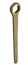
|
Figure 14 shows a box wrench. It works very well
for a particular size of nut or bolt. However, is doesn’t work at all
if the size is different by any significant amount.
|
|
Figure 15 shows an adjustable wrench. It can be adjusted to
fit a wide range of differently-sized nuts or bolts. However, it is
much bulkier and heavier than a comparably-strong box wrench.
|
Once again, the moral of the story is: Sometimes you want something
that applies to a specific case ... but sometimes you want something
that can be adjusted to cover a wide range of cases.
We can apply the same logic to mathematics. The variable x in
equation 29d and the variable S in equation 30
correspond to the worm gear in the adjustable wrench: They allow the
equation to be adjusted to cover a wide range of examples.
This idea gets used over and over again, to express all sorts of
mathematical principles. Let’s consider a few more examples:
-
In first grade or maybe in kindergarten,
you learned that 2+7 is equal to 7+2. It is also true that 3+7
is equal to 7+3. There are infinitely many examples of this kind.
It would be absurd to try to learn all the examples one by one. The
sensible approach is to learn the general rule.
- The less-good option is to say “addition is commutative”.
Alas, that doesn’t mean anything unless you already know what
“commutative” means.
- The better option is to use the language of algebra. We can say
that X+Y equals Y+X, for all real numbers X and Y. In this
way, we can use algebra to define what we mean by
“commutative”.
Note that the word “commutative” comes from the same Latin root as
the word for “commuting” to and from work. The core meaning is
“back and forth”. When we write that X+Y equals Y+X, it means
that the addition can be done left-to-right or right-to-left.
Here are yet more examples of rules that can be adjusted to cover a
huge number of examples:
-
For all real numbers X and Y,
we have X·Y = Y·X. In other words, multiplication is
commutative (when applied to real numbers). For example, 3·7 =
7·3.
-
Beware that most things in
this world are not commutative. Putting on your shoes does not
commute with putting on your socks.
Even multiplication is not necessarily commutative. U×V is
not generally equal to V×U if U and V are vectors or
matrices.
-
For all real numbers X, Y, and Z, we have
In other words, multiplication distributes over addition. For
example, 2·(3 + 7) = 2·3 + 2·7. In more detail:
|
2·(3 + 7) | | = | | 2·10 | | doing the addition first |
| | | = | | 20 |
| 2·(3 + 7) | | = | | 2·3 + 2·7 | | using the distributive law first |
| | | = | | 6 + 14 |
| | | = | | 20
|
| (32)
|
The distributive law (equation 31) is not primarily a
statement about the numbers X, Y, and Z. Rather it is a
statement about the multiplication operator, the addition operator,
and the relationship between them. This is discussed in more detail
in section 4.5.
Talking about operators involves some abstraction. It is not,
however, a very tricky kind of abstraction. Young children are good
at using abstraction, generalization, and symbolism in this way; they
do it routinely. Even a toddler playing with a doll is using a great
deal of symbolism and abstraction; everybody knows that the doll is
not a real baby; it is just a symbol representing a baby.
One reason for studying algebra is to learn more systematic ways of
using symbolism, abstraction, and generalization.
5.4 Algebra Can Express Dimensions and Units of Measurement
Let’s continue the discussion of dimensions and units that began with
example 1-2, example 1-3, example 1-4, and example 1-5. Here’s
another example in the same vein:
-
Suppose you cover five acres of land with water, to
a depth of 0.5 feet. That is 2.5 acre·feet of water. (This is
sometimes written as 2.5 acre−feet, but it is safer to write it as
acre·feet, with a dot rather than a hyphen, to remind everyone
that we are multiplying, not subtracting.)
Obviously, multiplying 5 acres by 0.5 feet requires multiplying 5 by
0.5 ... but it also requires multiplying acres by feet. Units (such
as acres and feet) are known quantities, but the rules for multiplying
known quantities are exactly the same as the rules for multiplying
unknown quantities such as X and Y.
In this way, algebra gives you systematic methods for converting
acre·feet to cubic feet, and then converting cubic feet to
liters, and so forth, to obtain whatever units of measurement you
like. It also tells you that cubic feet are dramatically different
from square feet, which is something worth knowing.
The general topic of how to keep track of dimensions and units of
measurement is called Quantity Calculus. It might have made
more sense to call it Unit Algebra or something like that, but the
experts tend to call it Quantity Calculus. A highly condensed
overview of the subject can be found in reference 12.
It is entirely possible to measure something using no units at all.
On more than a few occasions I have been miles away from the nearest
ruler, so I recorded in my notebook that something was
|——| long. That’s an analog measurement.
Physical quantities exist whether you measure them or not. In
particular, they exist independent of whatever units (if any!) you use
to measure them. In figure 1, the length of the hallway is
the same, no matter whether you measure it in meters, yards, feet,
cubits, or whatever. In particular, the length of the hallway is not
«L feet» or «L yards» or anything like that; the length is
simply L.
It is important to distinguish the dimensional quantity L from the
dimensionless ratio L/ft. Sometimes you want one or the other,
depending on circumstances.
Sometimes the penalty for getting the units wrong is on the order of
three hundred million dollars, as in the case of the Mars Climate
Orbiter (reference 13 and reference 14).
./img48logo-98t-s.png
Note that most calculators and old-school computer languages can
represent dimensionless numbers but do not automatically keep track of
the units. This creates all sorts of problems and risks. However,
with a modest amount of manual labor, it is possible to keep track of
the units, even under adverse circumstances, as follows:
Constructive suggestion: When using an old-school computer
language, we can use variable names of the form L__ft and W__yd,
where the convention is that the double underscore means “measured in
units of” and also “divided by”. (Let’s be sure to document this
convention.) This allows us to write things like the following. The
first line makes use of the fact that an inch is officially defined to
be 2.54 centimeters:
        in__m = 0.0254;         /* exactly, by definition */
        ft__m = 12 * in__m;     /* definition of foot */
        yd__m =  3 * ft__m;     /* definition of yard */
        L__m  = 10 * yd__m;     /* length of hallway */
        L__ft = L__m / ft__m;   /* length of hallway, in feet */
Example 1: Units, Using Old-School Computer Language
Another possibility is to use a computer algebra system. That means
that instead of the code in example 1, we can write code
like the following:
        L : 3 * yd;     /* length of hallway */
        yd : 3 * ft;
        ev(L);          /* result should be:  9 ft */
Example 2: Units, Using Computer-Algebra System
As far as the computer-algebra system is concerned, yd and
ft are algebraic abstractions, with no numerical value.
| Mutations: Non-experts should skip this
section. It discusses how things should not be done. I almost
hate to mention this, because discussing misconceptions is as likely
to spread them as to dispel them.
It is an all-too-common blunder to write something like
|
| |
☠ y | | = | | 10 | (the «yardage») | ☠ | |
(33a)
|
|
| |
☠ f | | = | | 30 | (the «footage») | ☠ | |
(33b)
|
|
| |
☠ f | | = | | 3 y | | ☠ | |
(33c)
|
|
The contrast between 1 yd = 3 ft and f = 3 y could not be more
extreme. That is the contrast between equation 3 and
equation 33c.
There are several things wrong with equation 33.
The whole approach is misguided. One problem is that if the length of
the hallway is y = 10, what is the width? Another problem is that
units should be on the RHS of the equation, or in the denominator of
the LHS, whereas the expression y = 10 seems to imply that the units
are in the numerator on the LHS – which is crazy backwards.
As previously mentioned, you can solve both of those problems by
writing things like L/yd = 10 and W/ft = 6. This allows us to
think clearly about the distinction between the dimensional quantity
L and the dimensionless ratio L/yd. |
5.5 Algebra Reduces the Amount of Stuff You Must Learn
The term “equation hunting” usually refers to a bad habit that
students sometimes pick up. For any given problem, they run down the
list of equations that they know until they find one that seems to
fit. They use this to solve the end-of-chapter problems in the
textbook. The only reason it appears to work is that there are
relatively few equations in the chapter, and all the end-of-chapter
problems can be solved using those few equations.
In contrast, this trick is not nearly so useful in the real world,
because the number of equations that you would have to consider is
ridiculously large.
Instead, for most purposes, the recommended procedure is to learn a
relatively small number of equations ... plus the rules of algebra.
The remembered equations rarely fit the given problem directly, but
can be transformed by algebraic means into something that does fit.
There is a real-world version of equation-hunting that actually works,
although it is very inefficient. Sometimes it is possible to guess
the exact form of the desired equation. Somewhat more often, it is
possible to guess that the desired equation belongs to a certain
family, and then systematically find which member of the family does
the job. In all cases the rule is that it’s OK to guess, provided you
check and confirm that the guess actually works. It’s not
guess-and-hope, it’s guess-and-check.
For example, Galileo equation-hunted the equation of motion for a
freely-falling object. He did not derive it. There was nothing he
could have derived it from. He conducted a long series of meticulous
experiments to confirm that his formula was correct, and that the
previous “conventional wisdom” was wrong.
Similarly, Newton equation-hunted the law of universal gravitation.
He did not derive it. There was nothing he could have derived it
from. He checked that it was consistent with Kepler’s laws, which in
turn were consistent with Tycho’s meticulous observations.
Similarly, Planck equation-hunted the first quantum mechanical
formula, the black-body spectrum. He did not derive it. There was
nothing he could have derived it from. He checked that it fit the
facts.
It must be emphasized that real-world equation hunting is very much
harder that end-of-chapter equation hunting. The number of
possibilities is very much larger. The required amount of
subject-matter expertise is very much larger. It might take years to
hunt up the desired equation.
Bottom line: Equation-hunting is a tool. Like any other tool, it
should not be over-valued or under-valued.
5.5.1 Density Formulas
In physics and chemistry, the density (ρ) is defined to be mass
(m) per unit volume (V):
|
ρ | | = | | m / V | | for all ρ, m, and V
|
| (34)
|
Using the laws of algebra, we can rearrange things in various ways.
For all ρ, m, and V we have:
|
| |
ρ | | = | | m / V | |
(35a)
|
|
| |
V | | = | | m / ρ | |
(35b)
|
|
| |
m | | = | | ρ V | |
(35c)
|
|
The point here is that a person who understands algebra sees
equation 35a, equation 35b, and equation 35c as all the
same. In contrast, a person who doesn’t understand algebra sees
equation 35a, equation 35b, and equation 35c as three
different equations, and must learn each of them separately. This is
three times as much work. It also means there are three times as many
things that could go wrong.
Here’s another example: In an ideal gas, there is a relationship
involving four variables: the pressure (P), volume (V), number of
molecules (N), and temperature (T). There is also a constant
involved, namely Boltzmann’s constant (k).
|
P V | | = | | N kT | | (ideal gas law)
|
| (36)
|
There are numerous possible rearrangements and corollaries to this
law. One of the corollaries is called Boyle’s law, but I don’t know
which one. Other corollaries are called Charles’s law, Avogadro’s
law, Gay-Lussac’s law, but I don’t know which is which. Some of the
other corollaries might have names, but I don’t even know the names.
I don’t need to know any of that stuff, because I know equation 36, and I can rederive the corollaries whenever needed, in less
time that it takes to tell about it, using simple algebra.
|
Each of the corollaries is predicated on certain assumptions,
and the assumptions are different in each case. So not only do you
need to memorize the equation for each corollary, you need to memorize
the assumptions. The number of hard-to-learn and easy-to-forget
details is astronomical.
|
|
The general law (equation 36)
easier to learn, harder to forget, and more reliable ... not to
mention more powerful.
|
5.5.3 Electronics Laws
This brings to mind a morbidly amusing story, as recounted by Joseph
Bellina:
| After graduating from
college and ROTC, this fellow chose to go to the Army
electronics school. As a pretest he was asked what are the
three most important laws of electronics. Well he thought
about that a while and chose j = σ * ρ, and
Kirchoff’s two laws. As it happened what they expected was V
= IR, I = V/R and R = V/I. |
The point here is that if you know a little bit of algebra, you see
Ohm’s law as one fundamental law, but if you don’t, you have to learn
it as three separate not-so-fundamental laws. Actually it’s even
worse than that, exponentially worse, as we now explain.
Let’s start from the beginning. In electronics, there is a
relationship involving the voltage (V), the the current (I) and
the resistance (R):
Using the laws of algebra, there are three ways of rearranging this:
|
V | | = | | I·R |
| I | | = | | V / R |
| R | | = | | V / I |
| (38)
|
So you have a choice: You can either remember three things
(equation 38) or you can remember just one thing
(equation 37) and use algebra to derive the others whenever
needed.
If that were the end of the story, the choice wouldn’t matter much.
Learning three things is not very much harder than learning one thing.
However, that’s not the end of the story. There is also an equation
for the power:
|
P | | = | | I·V | | (Joule heating law)
|
| (39)
|
Using the laws of algebra, there are 12 different ways of combining
equation 39 with equation 37 and rearranging things. Would
you rather learn 12 equations, or just 2 equations?
Note the trend here: The number of variables went up modestly, from 3
to 4. The number of basic concepts went up modestly, from 1 to 2.
The number of derived equations went up explosively, from 3 to 12.
Let’s take this one more step: We introduce the notion of conductance.
It’s an exceedingly simple concept:
This allows us to write things like I = G·V, which makes at
least as much sense as Ohm’s law in its original form. Now the number
of variables goes up from 4 to 5, and the number of basic concepts
goes up from 2 to 3. The number of equations continues its explosive
growth: It goes up from 12 to 24. Would you rather learn 24
equations, or just 3 equations?
|
If you count all the rearrangements, there are a huge number
equations. You could try to learn them by rote, but I don’t recommend
it. Real-world professional electronic engineers don’t know them all
by heart. The details are so gory that they are not shown here. You
can look at section 13.2 if you dare.
|
|
|
|
They actually sell posters for the benefit of people who
don’t understand algebra, to help them learn by rote all 12 possible
rearrangements of equation 37 in combination with
equation 39. Such a poster is shown in figure 17.
|
|
If you understand algebra, you don’t
need a poster covered in equations. As soon as you learn the basic
concepts, you get all the rearrangements for free.
|
At some point it becomes easier to just learn algebra than to do
everything using brute force and rote memory.
 Figure 17
: Poster for Learning Electronics Equations by Rote
5.5.4 Thermodynamics
In thermodynamics, the description of even a rather simple system
might involve a dozen variables and more than a dozen equations.
That gives rise to thousands of permutations and combinations – far
more than anyone could remember.
5.6 Algebra Can Find Solutions to Equations
Whenever you mention algebra, people think of methods for solving
equations. That is, sometimes you will know an equation for X
before you know the exact value of X, and then in a later step you
solve the equation to find X.
| It must be emphasized
that solving for the value of a variable is not the only thing
algebra can do. This is an important part of algebra, but
definitely not the only part. In particular, none of the examples
in section 5.3 involve solving for X. The power
of those examples comes from the fact that the equation holds
for any and all X. Furthermore, there are lots of situations where you are looking for
a solution, but it cannot be found using algebra alone. Sometimes
fancier techniques are needed, such as differential equations.
|
Solving equations has an enormous range of applications. For example:
-
Suppose you know the stopping distance for a car at
50 miles per hour. You also know the stopping distance at 10 miles
per hour. You would like to know the stopping distance at various
other speeds. The brute-force solution would be to measure the
stopping distance at every possible speed, one by one, and tabulate
the results.
The cleverer approach would be to use physics (including algebra) to
build a mathematical model. This allows you to interpolate, so you
know the stopping distance even at speeds that you didn’t explicitly
measure. What’s even better is that subject to mild restrictions,
you can extrapolate the model to speeds that you simply could not
measure, perhaps because of speed-limit laws, or because of the car’s
performance limits, or because they involve weather conditions that
you have not yet experienced, or whatever.
If we want to account for other variables that could increase the
stopping distance, such as a downhill slope or a tailwind, the
brute-force approach becomes even more impractical, and the
advantages of the mathematical approach become even more apparent.
Lives depend on getting this right. Note that in all likelihood, the
rule of thumb that they taught you in driver’s-ed class is not
reliable; it provides excessive margin under some condition and not
enough margin under other conditions. Knowing a little bit of
algebra allows you to figure this out.
-
As a more dramatic example, suppose you are in
command of a boat or an aircraft. You would be well advised to
calculate the amount of fuel required for the journey. You would be
wise to calculate it before departure, because you can’t get more
fuel in the middle of the ocean. At the very least, you have to
calculate it before you reach the point of no return. There
are plenty of situations like this, where making a direct measurement
is not a viable option.
-
Farming is tens of thousands of years older than
algebra, but modern farming is intensely analytical. Here’s a
simplified example: You can use a small test plot to experiment with
the amount of water, and another to experiment with the amount of
fertilizer, and another to experiment with pesticides, et cetera.
Then you need to interpolate and extrapolate all the variables, in
order to apply the results to your large main fields. There are so
many variables that you could not possibly find the right answer by
brute-force experimentation.
-
Suppose you have a talent for making exceptionally
good cookies. You decide to go into business. The question is, how
much should you charge for your cookies? You know how much the
ingredients cost. You know how much your competitors are charging,
but that doesn’t answer the question, because their costs are
different and their product isn’t as good. A small-scale experiment
tells you that if the price is too high, the sales-volume goes down
and you lose money. On the other hand, if the price is too low you
lose even more money.
If you are lucky, you may be able to use brute-force trial-and-error
methods to find a price that allows you to stay in business ... but
you will do better if you use algebra to analyze the data and
find the optimal price-point.
A modern high-efficiency outfit such as Walmart makes decisions based
on fantastically complex mathematical models.
6 More about Functions
6.1 Tabular and Graphical Approaches
The topic of this section is functions.
As mentioned in section 2.5, a great deal of mathematics
(especially higher mathematics) is devoted to patterns, relationships,
and generalizations. A function is a particular type of relationship.
Functions can be represented in many ways, including graphs, tables,
and algebraic expressions.
As a simple example, let’s take a look at table 7. This
is what we call a lookup table. The first column (Tc) is the
temperature in degrees Celsius. The second column (Tf) is the
temperature in degrees Fahrenheit. For the moment, let’s treat the
third column as a mere comment and ignore it.
| | | | Application |
| 0 | | 32 | | water: freezing point |
| 5 | | 41 | | |
| 10 | | 50 | | |
| 15 | | 59 | | |
| 20 | | 68 | | |
| 25 | | 77 | | |
| 30 | | 86 | | |
| 35 | | 95 | | |
| 37 | | 98.6 | | body temperature |
| 40 | | 104 | | |
| 45 | | 113 | | |
| 50 | | 122 | | |
| 55 | | 131 | | |
| 60 | | 140 | | |
| 65 | | 149 | | |
| 70 | | 158 | | |
| 75 | | 167 | | |
| 80 | | 176 | | |
| 85 | | 185 | | |
| 90 | | 194 | | |
| 95 | | 203 | | |
| 100 | | 212 | | water: boiling point |
Table 7: Temperature Conversion Lookup Table
Given a lookup table such as this, you can convert a temperature
reading from one scale to the other. For example, if the temperature
is represented as 10 ∘C, you can find that the corresponding
representation is 50 ∘F. This is the third row of the table.
This data can also be represented as a graph:
For some types of data, a table is the best representation. For other
types, a graphical representation might be helpful. However, for
temperature conversion, neither of these is optimal. The problem is,
there are lots of different temperatures in the world, and no table
can include all of them in any reasonable way. For example:
- Suppose you want to store some ice cream. The instructions
say to store it at -20 ∘C. How do we represent that
in Fahrenheit? The table doesn’t say.
- Suppose you want to cook a rib-eye roast. The instructions
say to heat the oven to 175 ∘C. How do we represent that
in Fahrenheit? The table doesn’t say.
- Suppose you are running a slight fever, with a temperature of 38
∘C? How do we represent that in Fahrenheit? The table doesn’t
say exactly. By looking at the table you can figure out that the
answer is “somewhere” between 98.6 and 104 ∘F, but to get more
accuracy would require a bunch of calculations ... or a better
graph, as we discuss below.
To solve the problem, you could interpolate and extrapolate.
There are various ways of doing this.
- One option would be to interpolate numerically. This definitely
requires algebra. It requires the use of a nontrivial algebraic
formula.
- You could draw the graph, and interpolate graphically. This
does not require any algebra – indeed it hardly requires any
arithmetic – but it is one of the things they teach you in algebra
class. Some schools have a so-called “pre-algebra” class that
covers stuff like this.
If you want to use the function in table 7 in the medical
clinic, you should plot the function, but the whole thing as shown in
figure 18. You need a more zoomed-in version, such as
shown in figure 19.
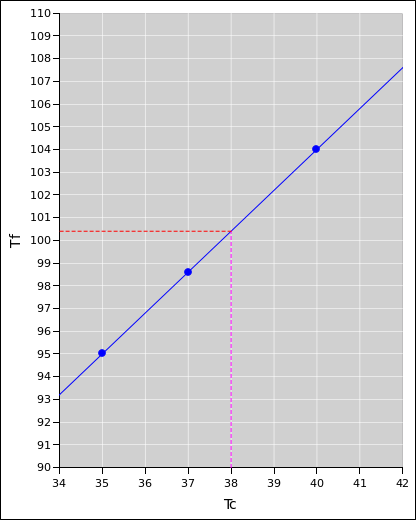 Figure 19
: Zoomed-In Temperature Conversion Graph
You can construct such a graph by hand, as follows: Take a piece of
graph paper. Select a suitable region, and label the grid-lines
more-or-less as shown in figure 19. Plot two of the
points from table 7, namely the points at (35, 95) and
(40, 104). Then draw a straight line connecting them and extending
beyond them a little ways in both directions. You don’t absolutely
need the intermediate point at (37,98.6), but it is a good idea to
plot it anyway, as a check. Remember the rule: Check the work.
This figure can be used for interpolation of clinically-relevant
temperatures. For the example of 38 ∘C, find the contour labeled
38 ∘C, and follow it. This is a contour of constant Tc. It
contour runs vertically in the figure, and is shown by the magenta
dotted line. Follow it this contour until you come to the line that
represents the temperature-conversion function. Then follow along a
contour of constant Tf. This runs horizontally, and is shown by a
red dotted line in the figure. Follow it until you run into a label.
You can see that it is a little less than halfway between 100 ∘F
and 101∘F. In fact it is exactly 100.4 ∘F, as we can
confirm using algebraic methods as discussed in section 6.2.
The spreadsheet that produces these figures is cited in reference 15.
Beware that extrapolation is always riskier than interpolation.
Being able to construct and interpret graphs is an exceedingly
valuable skill. Math gets a lot more interesting and a lot more
useful as soon as you move beyond arithmetic. It is very hard to see
the significance of a pile of numbers just by looking at the numbers.
Doing more and more arithmetic with the numbers is not going to help.
Graphic the numbers helps a lot.
6.2 Algebraic Approaches
At some point it becomes easier to ignore the table and calculate the
conversion from scratch, using an algebraic formula. The formula for
converting Celsius to Fahrenheit is nice and simple:
That’s an equation. It says the left-hand-side (LHS) and the
right-hand-side (RHS) are equal, which is true.
However, there is something more going on here, which we can write as
follows:
The arrow in recipe 42 means the LHS is calculated
from the RHS. This is an algebraic rule, a machine if you will.
Given a Tc value, this machine performs some mathematical
manipulations and spits out a Tf value.
Note the following contrast:
|
When writing a lookup table, it is more-or-less traditional
(but certainly not necessary) to write the input in the left column
and the output in the right column, so that the table can be read
left-to-right.
|
|
When writing instructions for calculating something,
there is a very strong tradition of writing the output on the left and
the expression that involves the inputs on the right. You can see
this in recipe 42 and also in figure 20.
This may seem backwards to you, but there is no point in fighting it.
|
Note that the entries in a lookup table do not need to be evenly
spaced. You can see this in table 7: There are
unevenly-spaced entries near 37 ∘C.
6.3 More Examples
Indeed, the entries in a lookup table do not need to be sorted
numerically, or even sortable. Indeed, they do not even need to be
numerical. For example, the data in table 3 is
non-numerical.
Table 8 shows another example of a function.
| | |
| −5 | | 25 |
| −4 | | 16 |
| −3 | | 9 |
| −2 | | 4 |
| −1 | | 1 |
| 0 | | 0 |
| 1 | | 1 |
| 2 | | 4 |
| 3 | | 9 |
| 4 | | 16 |
| 5 | | 25 |
Here is the algebraic form of this function:
Figure 21 shows the corresponding graph.
6.4 Inverse Functions
Table 7 can be used in either direction. So far we have
treated the first column as the input and the second column as the
output, but you can perfectly well use the table in the other
direction. For example, if the temperature is represented as 50
∘F, you can find that the corresponding representation in 10
∘C. This gives us a new machine, a new function. We
can write it algebraically as:
The function in recipe 44 is called the inverse of
the function in recipe 42.
We can convert recipe 44 to an equation:
Note the contrast:
|
Equation 45 means exactly the same thing as
equation 41. If one of them is true the other must be true.
|
|
Recipe 44 is not the same as Recipe 42. One
recipe says to use Tc to calculate Tf, while the other says to
use Tf to calculate Tc.
|
|
An equation states that the LHS is equal to the RHS and vice
versa; it’s all very symmetrical.
|
|
In a function, the input is
conceptually different from the output. There’s nothing symmetrical
about it.
|
Interestingly enough, it is not quite so easy to form the inverse of
the function in table 3. That’s because for any given
color, there are multiple kinds of fruit with that color.
For the same reason, it is not entirely simple to form the inverse of
the function in table 8 aka figure 21 aka
equation 43.
Mathematicians are quite strict about this: For any given input-value,
a function has to produce the same output-value every time. A machine
that doesn’t obey this rule is not a function.
There are lots of things in this world that aren’t functions. For
instance, a clock gives you a different answer every time you look at
it. It’s a perfectly good clock, but it’s not a function.
Sometimes when you have a relationship that is not a function, you can
turn it into a function by gathering things into sets. Table 9 is a machine that takes in a color and produces a
set of fruits that have that color. This is not exactly the
inverse of the function in table 3, but it is a perfectly
fine function unto itself.
| color | | set of fruit |
| yellow | | {banana, lemon} |
| red | | {cherry, McIntosh} |
| green | | {lime, Granny Smith} |
Table 9: Fruit as a Function of Color
Similarly table 10 is a machine that takes in a s-value
and produces a set of r-values that are consistent with that s
value, and consistent with the requirement that s = r2. This is
not exactly the inverse of the function in table 8, but it is
a perfectly respectable function unto itself.
| | |
| 0 | | {0} |
| 1 | | {1, −1} |
| 4 | | {2, −2} |
| 9 | | {3, −3} |
| 16 | | {4, −4} |
| 25 | | {5, −5} |
Figure 22 shows the corresponding graph.
It must be emphasized that even though there is an inverse function
for the temperature conversion function in table 7, there
is no inverse function for the fruit/color conversion in
table 3. The inverse function would completely undo the
effect of the fruit/color conversion machine, but this is simply not
possible. The output of the fruit/color conversion machine contains
less information than its input.
Similarly there is no inverse function for the squaring function in
table 8. The inverse function would completely undo the
effect of the squaring machine, but this is simply not possible. The
output of the squaring machine contains less information than its
input.
Sometimes it is satisfactory to have a function that spits out a set
of numbers (or a set of fruit), but sometimes not. If you are
building a machine for use in grocery stores that figures out the type
of fruit, it won’t be very useful if it can’t tell the difference
between a cherry and a McIntosh. You need a more complicated
function, with more inputs. The color information is still useful as
part of the overall solution, but it is not a complete solution unto
itself.
A set of ordered pairs is called a mapping. Every function is
a mapping, but not conversely. A function is required to have a
unique output for any given input, but a mapping has no such
restriction. Every mapping has an inverse mapping, but not every
function has an inverse function. The inverse function is required to
completely undo the effects of the original function, but an inverse
mapping has no such requirement.
Figure 21 is a function that converts one number to
another. It is also a mapping.
Considered as mappings, figure 22 is the inverse of
figure 21. Considered as functions that convert one
number to another, figure 22 is not a function at
all.
6.5 Graphing Inverse Functions
In item 4-5 we encountered the following graphs:
It must be emphasized that these two figures convey exactly the same
information. If you prefer one over the other, that is mostly a
matter of personal taste.
Anything you can do moving horizontally in one figure you can do
moving vertically in the other, and vice versa. In fact, you draw
figure 23 on a transparent piece of plastic, you don’t
need to draw figure 24 at all; you can just flip
figure 6 over and look at its back side. You can flip
it left-to-right or top-to-bottom and then rotate it into position.
You don’t even need the rotation step if you flip it around a 45∘
diagonal, as shown in figure 25.
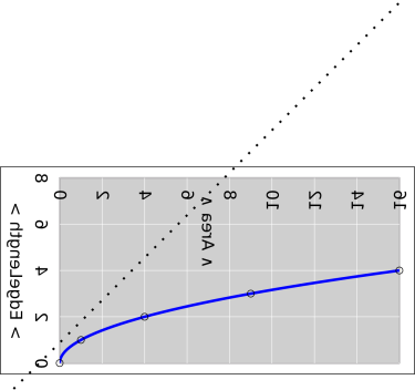 Figure 25
: Inverted View of Area versus EdgeLength
Equivalently, you can produce the image of figure 25 by
viewing figure 6 in a mirror. The labels are hard to
read because they are mirror-inverted, but the data itself is plotted
correctly.
You can even combine the plot with its mirror image to create
symmetrical “butterfly” diagrams. An example is shown in
figure 26. There is something fundamentally hokey
about this example, because we have two different coordinates (both
length and area) in each direction. In real life it is rare to find a
mapping where its range is more-or-less the same as its domain ... but
it does happen. In such a case, the flipped diagram can be thought of
as a representation of the inverse mapping.
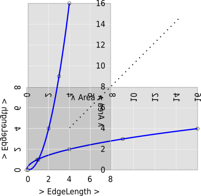 Figure 26
: Combined View of Area versus EdgeLength
However, this is not necessarily the best way to
think about inverses. When the range is not similar to the
domain, as in the fruit/color function in table 3,
there is no simple geometrical symmetry, and otherwise just causes
confusion.Figure 27 is perhaps a better way of visualizing
the symmetry between a function and its inverse. Enter one of the
plots and move vertically along the dashed line that represents
Area=7. When you come to the curve, move horizontally along the
dashed line that represents EdgeLength=√7. Carry this
across to the other plot, and keep moving horizontally. When you
get to the curve, move vertically along the dashed line that
represents EdgeLength=7. The overall result is a graphical
computation of (√7)2.
In figure 27 you may well ask, which plot
represents the function and which represents the inverse? Answer:
Whichever you choose. The point is, on one plot you enter
vertically and read off the answer horizontally, while on the
other plot you enter horizontally and read off the answer
vertically. Each function is the inverse of the other.
Figure 28 is perhaps an even better way to
visualize the relationship between a function and its inverse.
This version will appeal to those who like the input of a function
to run horizontally and the output to run vertically.
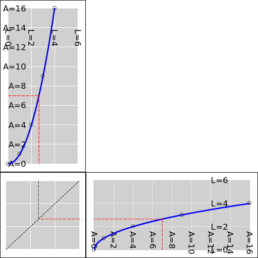 Figure 28
: A Function and its Flipped Inverse
Enter the lower-right diagram and run vertically along the dashed
line that represents Area=7. When you get to the curve
representing the function, pivot and run horizontally along the
dashed line that represents EdgeLength=√7.
Continue this onto the “reflector” panel. Pivot and vertically
run along the dashed line that – still – represents
EdgeLength=√7. When you get to the curve representing the
function, pivot and run horizontally along the dashed line that
represents Area=7. The overall result is another graphical
computation of (√7)2.
The “reflector panel” plays an important role here. It
represents the identity function, in a way that lines up the
output of one function with the input of the next. I think it
helps to show it explicitly.
The “reflector panel” trick can be used to diagram a graphical
computation of the composition of any functions (not just
inverses), so long as the range of one matches the domain of the
next. Lay them down like dominoes.
Sometimes the range and domain are the same. For example, a
permutation is guaranteed to have a range identical to its
domain. Whenever the range of some function f is a subset of the
domain, we can write equations of the form
which we call an iterated mapping. This includes the case where
the range is an improper subset of the domain, i.e. the whole
thing. In the opposite case, where the range is systematically
smaller than the domain, we get what is called a contractive
mapping.
The spreadsheet that produces these figures is cited in reference 15.
6.6 Equations versus Recipes, Causation, etc.
Note the contrast:
|
In some sense, there is a profound distinction between an
equation and a recipe. An equation is symmetrical, in that the LHS is
equal to the RHS and vice versa.
|
|
In another sense, the distinction
between an equation and a recipe does not matter much, because any
recipe can be converted into an equation, and a wide class of
equations can be converted into recipes. Many of the same algebraic
operations that can be applied to equations can be applied to
recipes.
|
A lot of people, including experts, tend to gloss over the distinction
between equations and recipes. An assignment statement in an
imperative computer language such as C++ is written with an equals
sign, even though it logically should be written with an arrow or with
a “:=” symbol. It “looks like” an equation, and is sometimes even
called an equation, even though it really isn’t. There is no symmetry
between the LHS and RHS of an assignment statement.
For more about symmetry (or the lack thereof) as applied to equations,
assignments, and cause-and-effect relationships, see
reference 16.
6.7 Conventional Directions and Symbols
As mentioned in reference 10, introductory textbooks tend
to fall into the following habits:
- ☠ Supposedly, x is always the input and y is
always the output.
- ☠ Supposedly, on a graph, x is always horizontal
and y is always vertical
- ☠ Supposedly, on a graph, the input is always
horizontal and the output is always vertical.
In mathematics, none of those things is actually required. You
should break those habits. (Some spreadsheet apps force on you the
idea that the horizontal direction is called x and the vertical
direction is called y, but it is still a bad idea.)
For example, you can use figure 18 to convert Tf to
Tc just as easily as vice versa. You don’t even need to redraw
the graph; just start with a Tf value, move horizontally until you
come to the curve, and then move vertically to find the label for the
corresponding Tc value.
7 Some Fancier Applications
The goal is to understand some useful applications. We start by
describing the applications. We then work backwards, developing the
techniques necessary to solve the problem. We then go over everything
again tidying up loose ends. This is an example of the spiral
approach to learning and problem-solving. It has advantages in terms
of motivation as well as realism, as discussed in reference 17.
7.1 Saggy Suspension Bridge (Setup)
Suspension bridges are important in the real world. People have been
building them for thousands of years. Unfortunately, if you build
them in the most obvious naïve way, they either sag or break.
Not too long ago, the Mythbusters discovered this the hard way. They
built a suspension bridge. They discovered that it sagged, as shown
in figure 29. The desired result is shown by the
horizontal dotted black line, while the actual result is shown by the
saggy solid red line. They could reduce the amount of sag by
increasing the tension, but too much tension would cause the thing to
break. It was a no-win situation: either too much sag or too much
tension, or both.
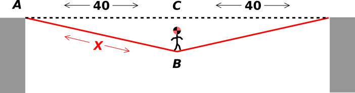 Figure 29
: Crash Test Dummy Crossing a Bridge
Just to be silly, they built the bridge out of duct tape, but that is
irrelevant to our story. Any other material would have had the same
problem. This problem has been around for thousands of years.
The engineering problem can be understood in terms of physics, which
can be understood in terms of geometry, which can be understood in
terms of algebra.
|
engineering → physics → geometry → algebra
(47) |
The basic physics idea is mechanical advantage. Leverage is a
familiar example of mechanical advantage. Screws and wedges also
provide mechanical advantage. The load on the bridge has mechanical
advantage against the rope. To say the same thing the other way, the
rope suffers from a large amount of mechanical disadvantage.
That’s because a small amount of stretch produces a disproportionately
large amount of sag.
Using the naïve design shown in figure 29 there
is no way to solve this problem. In the real world, suspension
bridges are built with tall towers supporting catenary cables. If you
want a deck that doesn’t sag, you can support the deck using vertical
suspenders that come down from the catenaries, as shown in figure 30. Physics demands that you must let
the catenaries sag! Something has to sag, because otherwise the load
has an infinite mechanical advantage.
 Figure 30
: Verrazano Narrows Bridge
./img48verrazano-narrows-bridge.jpg
In accordance with equation 47, before we can
understand the physics or the engineering, we need to understand the
geometry of the situation.
Rather than attack the engineering problem head-on, let’s start by
doing an easier problem that has the same geometry as figure 29. Algebra helps with this, as we shall see in
section 7.2.
There is an important strategic principle here: Sometimes when faced
with a hard problem it pays to work on an easier problem first. This
can be considered a form of reconnaissance.
|
It pays to do warm-up exercises.
|
|
|
|
We will finish the saggy-bridge problem in section 7.3. First, though, let’s work the navigation
problem in section 7.2. It has the same geometry as the bridge
problem, but with fewer distractions.
7.2 As the Crow Flies
7.2.1 Initial Rough Analysis
Suppose you are traveling from point A to point B in figure 31. In particular, suppose you are driving an all-terrain
vehicle in flat, open country, so you are not obliged to follow roads.
The same logic applies to airplanes and to birds, which are not
confined to roads. In all cases we keep things simple by ignoring
headwinds and crosswinds.
One option is to travel from A to C, make a 90∘ left turn,
and then proceed from C to B. The total distance for this route
is 49 miles.
Another option is to proceed “as the crow flies” from A directly
to B, as shown in red in the diagram. Everybody knows that a
straight line is the shortest distance between two points, but let’s
see if we can figure out how much shorter it is.
This is a legitimate problem unto itself, although not
ultra-important. The real significance comes from the fact that the
techniques used here are necessary for solving harder and more
important problems, such as suspension bridge problem in section 7.1.
At this stage we don’t have a numerical value for the distance, so we
call it X. You could just construct a mechanical model or a careful
scale diagram and measure X. Or you could travel the route both
ways and keep careful records. These are clumsy ways of discovering
X, but they work. If you do that, you find that X is
approximately 41 miles. People speak of “cutting corners”, and
this is why. The short-cut route saves a substantial amount of
distance: 41 miles is almost 20% shorter than 49 miles.
If you were in the delivery business, and your costs were 20% higher
than the competition, your business would fail very soon.
7.2.2 Mathematical Analysis
So, now that we are properly motivated, let’s see if we can find a
more-mathematical, less-clumsy way of finding the value of X. There
are lots of scenarios in which the mathematical approach works better
than the clumsy approach:
- Suppose you are only going to make the trip once or twice,
so you cannot afford the time and fuel it would take to check
every possible route experimentally.
- Suppose the trip is just barely possible, because of
limits on the size of your fuel tank, so you need to find
the optimal route in advance, and you need a highly accurate
estimate of the distance, more accurate than you could get
by measuring an analog drawing.
- Suppose you are transporting transplant organs, or some other
exceedingly perishable high-priority items. You need to calculate
the optimal route. You don’t have time to construct accurate analog
models, and you don’t have time to experiment with alternate routes.
- Suppose you are building a suspension bridge. It is a
tremendous waste of resources to build a bridge and then discover
that it sags or breaks or both. It’s also dangerous. Furthermore,
building an unsatisfactory bridge (as in figure 29) tells you that you have a problem, but doesn’t
necessarily tell you how to fix the problem. You need physics and
math if you want to understand why every bridge of the kind in
figure 29 suffers from some serious fundamental
limitations.
- Et cetera.
The mathematical approach uses the Pythagorean theorem
(equation 23). It tells us that:
You could work this out on a calculator, but just to prove a point let
me show how you could solve this problem in your head.
Let’s start with the numbers on the right-hand-side (RHS): 40 times
40 is 1600. You should be able to do that one in your head,
starting from the fact that 4 times 4 is 16. Similarly you know
that 9×9=81. So the number on the RHS of equation 48 is 1681.
So, if X squared is equal to 1681, then X itself is equal to the
square root of 1681, which we write as √1681. That is
Now, you could use your calculator to find the square root of 1681, but
again, you could also do it in your head. There are actually several
ways of doing it.
7.2.3 Taking the Square Root; Using the Binomial Theorem
One way of doing it is a two-step process. The first step is to guess
a value for X, and the second step is to prove that the guess is
correct. Since we have already guessed that X is approxmately 41,
let’s check to see if X=41 is mathematically correct.
As is so often the case, you can check this result by working the
problem in reverse. Just as you can check subtraction problems by
adding, you can check square-root problems by squaring. That is, if
we think X = √1681, we check it by showing that X·X =
1681.
It’s easy to multiply 41×41 in your head. Once again, algebra
comes to the rescue. Here’s how: We can write 41 as 40 + 1. Using
the language of algebra, we can rewrite that as (a + b) = 41, where
a = 40 and b = 1. To repeat:
|
a | | = | | 40 |
| b | | = | | 1 |
| (a + b) | | = | | 41
|
| (50)
|
The next step is easy if you know the following formula:
|
(a + b)2 | | = | | a2 + 2a·b + b2 | | (for all a and b)
|
| (51)
|
Equation 51 is a special case of the binomial theorem. It
is so widely useful that it is worth remembering. If you don’t
remember it, you can always re-derive it using basic algebra. The
derivation is shown in section 9.1.
Equation 51 is valid for any a and b whatsoever, which
means (among other things) that we can apply it to the a and b
values in equation 50.
|
| |
a | | = | | 40 | | | |
(52a)
|
|
| |
b | | = | | 1 | | | |
(52b)
|
|
| |
(a + b) | | = | | 41 | | | |
(52c)
|
|
| |
(a + b)2 | | = | | a2 + 2a·b + b2 | | (for all a and b) | |
(52d)
|
|
| |
| | = | | 402 + 2·40·1 + 12 | | (in this example) | |
(52e)
|
|
| |
| | = | | 1600 + 80 + 1 | | | |
(52f)
|
|
| |
| | = | | 1681 | | | |
(52g)
|
|
The multiplications called for in equation 52e are
super-easy because there is no carrying involved. Avoiding messy
carries is a big part of the rationale for what we did, expanding 41
into two terms and applying the binomial theorem.
7.2.4 Taking the Square Root; First-Order Expansion
Here’s another scheme for finding the square root of a number. This
scheme does not require guessing.
Here a simple yet powerful trick. It useful for solving this problem
and thousands of similar problems. There is a rule of thumb that says
if X goes up by one percent, X2 goes up by approximately two
percent. This rule is worth remembering, but if you ever forget it,
you can rederive it. The derivation and explanation can be found in
section 9.2.
We can apply this rule to equation 49 as follows. We
just got through calculating that 1600 is the square of 40, so we know
that 40 is the square root of 1600. Next we notice that 1681 is about
5% bigger than 1600. In particular, 1616 would be about 1% bigger,
1632 would be 2% bigger, et cetera. Since 80 is 16×5, and 81
is very nearly 80, we know that 1681 is very nearly 5% bigger than
1600. Since X2 is about 5% bigger than 1600, X itself must be
2½% bigger than 40. You can do that one in your head, too,
since 2.5% of 40 is just 1. So our estimate is that X=41.
Given an estimate like this, the first thing you should do is check
it. As in section 7.2.3, you can check it by
calculating X2 and comparing it to 1681.
7.2.5 Taking the Square Root; Newton’s Method
Suppose you didn’t know the trick for expanding things to first order
(as discussed in section 7.2.4) – or suppose for
some reason it wasn’t particularly convenient.
Here’s another trick, an incredibly powerful trick, invented by Sir
Isaac himself.
Suppose we start with X2 and divide by X. The quotient is
just X. That’s obvious.
Suppose we start with X2 and divide by something slightly smaller
than X. The quotient will be slightly larger than X. What’s
more, if the divisor is too small by a small percentage, the quotient
will be too big by the same percentage, to a good approximation.
Therefore if we split the difference, we obtain a very accurate value
for X.
We can say the same thing more precisely using the language of
algebra.
|
P | | = | | initial approximation, close to X |
| Q | | = | | |
| R | | = | | |
| | | = | | better approximation |
| (53)
|
If necessary, you can repeat the process, dividing X2 by R and
splitting the difference to get an even more accurate approximation.
The sequence converges rapidly. The number of correct digits doubles
each time. That is to say, if the initial approximation is good to
1%, one turn of the crank gives you an answer that is good to 0.01%.
Let’s apply this to the problem at hand. Suppose we don’t have a very
good guess for X. We still have some sort of guess; in
particular, we know that X has to be somewhere close to 40. You can
divide 1681 by 40 in your head. Write it as (1600 + 80 + 1) and
divide each term by 40. The answer is 42 to a good approximation.
It’s (42 + 1/40th) exactly, but let’s not bother with the
1/40th for now.
If you split the difference between 40 and 42, you get 41. You should
immediately check this. You will discover that it is in fact exact.
7.2.6 Discussion
This whole section has been something of a fugue, making some
low-level points and high-level points at the same time. Let’s
summarize:
|
Utilitarian Level
|
|
Intellectual Level
|
|
We have been discussing much distance you can save by taking
a short-cut, traveling as the crow flies. That’s slightly interesting
and slightly useful in practical terms.
|
|
Just calculating the
difference is not the whole point, or even the main point. The more
important lesson here is to see the mathematically-savvy way of
looking at such problems.
|
|
If all we wanted was a utilitarian solution, we could just
grind out the numbers on a calculator. There’s nothing wrong with
that.
|
|
The mathematician looks at this problem and says, not only can
we solve it, we can understand it.
|
|
If you solve lots of problems using a calculator, you get
good at using the calculator. There’s nothing wrong with that.
|
|
If
you solve the problem in your head, you get good at solving problems
in your head. To make it solvable, you need to understand the
structure of the problem, so you can rearrange and simplify the
calculations. This means you get good at understanding the
structure of problems. This is tremendously valuable.
|
|
If all you wanted was a solution, once you had a solution,
you’d be done.
|
|
To the mathematician, the problem is interesting.
Once you have a solution, you look for another solution, and then
another.
|
|
We used about ten different tools to attack this one little
problem. If all you wanted was one solution to one problem, ten tools
would be overkill. The time spent learning the tools wouldn’t be
worth it.
|
|
The same ten tools can be used to solve thousands upon
thousands of problems, including big problems as well as little
problems. Once you know the tools, you begin to see opportunities to
use them. No one particular problem makes the tools worthwhile; the
payoff comes from using the tools over and over again.
|
|
We have demonstrated how things work when a is equal to
some number and b is equal to some other number.
|
|
The idea of
turning a hard problem into a succession of easy problems by repeated
use of the distributive law comes up again and again and again. It
works just fine when applied to a tremendous variety of things,
including rational numbers, complex numbers, vectors, matrices, or
whatever – even if you don’t know what a and b stand for.
|
|
|
|
Equation equation 57d works on a wide range
of things. On the other hand, you have to be a little bit careful not
to apply equation 57e to situations where the
commutative law doesn’t apply (such as matrices and Clifford
algebras).
|
|
Calculating the optimal route is a toy problem. Everybody
knows that a straight line is the shortest distance between two
points.
|
|
If there are obstacles, or if you are living in a curved
space, it may not be obvious how to define “straight” line. In
particular, the surface of the earth has intrinsic curvature. As a
consequence, if you are using a map with a Mercator projection, a
straight line on the map – i.e. a rhumb line – is not the
shortest distance between two points. The tools exhibited here
(including the binomial theorem, expansion to first order, and
Newton’s method) can be brought to bear on real-world problems, such
as the suspension bridge in section 7.1.
|
7.2.7 Designing the Problem
In case it wasn’t obvious, I chose artful values (40 and 9) for the
perpendicular leg distances in section 7.2 to ensure that the
diagonal distance would come out to be a round number. I had to do a
few lines of algebra in order to know in advance that 40 and 9 would
work out nicely. So this in itself is an example of real-world
algebra: I had to do some real algebra just to set up the toy problem.
In particular, consider the case where we have a right triangle. We
require all the side-lengths to be integers. We require the
hypotenuse to be one unit longer than the base. We can use
algebra to find all such triangles.
|
| |
base | | = | | N | |
(54a)
|
|
| |
hypotenuse | | = | | N+1 | |
(54b)
|
|
| |
altitude | | = | | m | |
(54c)
|
|
| |
m2 | | = | | (N+1)2 − N2 | |
(54d)
|
|
| |
| | = | | 2N + 1 | |
(54e)
|
|
| |
2N | | = | | m2 − 1 | |
(54f)
|
|
| |
| | = | | (m+1)·(m−1) | |
(54g)
|
|
| |
N | | = | | (m+1)·(m−1)/2 | |
(54h)
|
|
Obviously 2N+1 is an odd integer, so equation 54e tells us
this only works for odd values of m. Otherwise it works for any odd
m larger than 1. Equation 54h is guaranteed to give us
an integer value of N, not a half-integer, because (m−1) is
guaranteed to be even.
Here are the first few triangles in this set:
|
| | altitude | | base | | hypotenuse |
| 3 | | 4 | | 5 |
| 5 | | 12 | | 13 |
| 7 | | 24 | | 25 |
| 9 | | 40 | | 41 |
| 11 | | 60 | | 61 |
| 13 | | 84 | | 85 |
| 15 | | 112 | | 113 |
| 17 | | 144 | | 145 |
| 19 | | 180 | | 181 |
| 21 | | 220 | | 221 |
|
(55) |
7.3 Saggy Suspension Bridge (Completion)
There is one tiny bit of physics we need to invoke in order to finish
the problem. To compute the mechanical advantage, we need to know how
the length of the rope changes as the amount of sag
changes. This makes sense if you look at it as follows: Suppose
you are using a lever, such as a crowbar or wrench. It doesn’t
directly matter where the handle starts or ends up; the thing that
directly factors into the mechanical advantage is how far the handle
moves, i.e. the distance from start to finish.
So let’s calculate what happens during the last part of the sagging
process, when the amount of sag goes from 8 feet to 9 feet. That’s a
one-foot change. We calculate that the length of each half of the
rope goes from 40.792 feet to 41 feet. That’s a 0.208 foot change in
each half of the rope, or 0.416 foot total. Taking the ratio of the
changes, we find that the mechanical advantage is about 2.4 to 1.
Looking at the next foot of sag, going from nine feet to ten feet, the
mechanical advantage is a little less.
Using calculus you could
figure out that a more accurate answer is 2.22-to-1
(assuming a 9-foot sag). It’s just 40 divided by 9,
divided by 2. However, that’s more than we really
need to know. You can solve this problem without
calculus. It’s more work and somewhat less exact, but
it’s entirely doable.
If you tried to reduce the sag to 4 feet, the mechanical advantage
would shoot up to five-to-one. This has some dramatic implications.
Suppose you wanted the useful load to be a few hundred pounds.
Multiply by the mechanical advantage, then multiply by some safety
factor, and you find that the strength of the rope has to be many
thousands of pounds.
To say the same thing another way, when the sag is 4 feet, the tension
is about worse than you might have guessed. The argument goes like
this: Given a certain amount of tension in an 80-foot rope, there will
be a certain amount of stretch. However, at the middle of the bridge
you are in effect being supported by two 40-foot ropes. Each one is
shorter (so there will be less stretch, for any given amount of
tension) and there are two of them (so there will be only half as much
tension in each rope). That’s all true as far as it goes, but it
would be a huge mistake to stop the analysis at that point. One must
account for the fact that changing the altitude of a triangle changes
the hypotenuse very little. All in all, rather than having a 4-to-1
advantage in favor of the rope, there is a 5-to-1 advantage in favor
of the load.
A graph of the mechanical advantage is shown in figure 32.
The raw numbers are shown in equation 56.
|
| | | | | | | | | | | | mechanical |
| horiz | | sag | | diagonal | | | | stretch | | advantage |
| 40 | | 0 | | 40.000 | | | | | | |
| | | | | | | } | | 0.012 | | 40.0 |
| 40 | | 1 | | 40.012 | | | | | | |
| | | | | | | } | | 0.037 | | 13.3 |
| 40 | | 2 | | 40.050 | | | | | | |
| | | | | | | } | | 0.062 | | 8.0 |
| 40 | | 3 | | 40.112 | | | | | | |
| | | | | | | } | | 0.087 | | 5.7 |
| 40 | | 4 | | 40.200 | | | | | | |
| | | | | | | } | | 0.112 | | 4.5 |
| 40 | | 5 | | 40.311 | | | | | | |
| | | | | | | } | | 0.136 | | 3.7 |
| 40 | | 6 | | 40.447 | | | | | | |
| | | | | | | } | | 0.160 | | 3.1 |
| 40 | | 7 | | 40.608 | | | | | | |
| | | | | | | } | | 0.184 | | 2.7 |
| 40 | | 8 | | 40.792 | | | | | | |
| | | | | | | } | | 0.208 | | 2.4 |
| 40 | | 9 | | 41.000 | | | | | | |
| | | | | | | } | | 0.231 | | 2.2 |
| 40 | | 10 | | 41.231 | | | | | | |
|
(56) |
8 Tools and Technques
8.1 Side Effects, or Not
Let’s take another look at the reasoning skills mentioned
in section 2.2.
| multi-step reasoning (section 8.2) | |
| higher reliability, stronger proof | |
| trusting certain tools | |
| avoiding certain booby traps | |
| skimming, reading, re-reading, and pondering a text (section 8.3) | |
| learning a new language | |
| generalization, symbolism, and abstraction | |
| imagination, creativity, artistry, and elegance | |
None of these things is intrinsically mathematical. For example,
computer programming requires just as much multi-step reasoning,
attention to detail, skimming, pondering, tools, symbolism,
linguistics, and creativity. On the other hand, traditionally,
through most of history, mathematical training has been the primary
means of acquiring these skills ... not universally, not necessarily,
but typically. The converse is a stronger statement: won’t be able to
handle higher math unless you learn these higher-order reasoning
skills. So these skills can be considered side-effects of studying
math.
These so-called side-effects are important. Most people don’t really
benefit from knowing how to derive the quadratic formula or prove the
Pythagorean theorem, but they do benefit from the reasoning skills
implicit in such exercises. So the tail is wagging the dog: The
side-effects of the math course are more important than the nominal
subject matter.
These side-effects are so strongly associated with mathematics that
some bureaucrats require an algebra course for reasons having precious
little to do with algebra. This is bad policy; it would be better to
directly require the things you care about. In particular, a computer
programming course could be used to impart all of the higher-order
reasoning skills listed above, and would be at least as practical.
Einstein said that an education is what remains after you’ve forgotten
everything you learned in school. That’s amusing, but in some sense
it is a symptom of bad pedagogy: It means the stuff you were
supposedly learning wasn’t what you were actually learning; the stuff
that was supposedly important wasn’t what was actually important.
8.2 Multi-Step Processes Require High Reliability
Suppose for example that you are given a quiz with 100 simple one-step
questions, and you get 94% of them correct. That sounds like a
pretty good score. Now in contrast, imagine a quiz with only 5
questions, each of which requires 20 steps. The overall number of
steps is the same as before – 100 steps total – but if each step has
only 94% reliability, you’d be lucky to get 2 of the 5 questions
right.
There are a lot of situations in real life where you have to handle
complex multi-step problems, and you do not get partial credit. If
you are driving a car on a crowded street and you manage to miss 95%
of the pedestrians, that is not considered an acceptable score. You
are required to miss all of them, all of the time.
Supoose you build a moon rocket with a million parts, each of which
has to work correctly. Then if each part is 99.9999% reliable,
there’s less than a 40% chance that the overall system will work. If
you want the overall system to be reliable, the failure rate for each
individual part has to be very much less than one part in a million
... and/or you need to arrange for some redundancy, so that if one
part fails another can take up the slack.
Similar logic applies to building a computer: It contains billions of
transistors. If you want the overall system to be reliable, the
requirements on the individual transistors are mind-bogglingly strict.
You should be wondering where that 40% number came from. More
precisely, it is 1/e = 1/2.71828 = 36.79%. It is an interesting
math exercise to work this out.
8.3 Skimming, Reading, Re-Reading, and Pondering
Nobody is smart enough to understand a math text on first reading.
Instead you have to start by skimming it. Then go back and read it
more carefully. Later, to back and re-read it.
There is nothing intrinsically mathematical about it. The same could
be said for physics books, for Russian novels, for sheet music, et
cetera. The notes on a sheet of music don’t tell you everything you
need to know; you have to interpret them.
Skimming means that when you come to something you don’t understand,
don’t panic, and don’t give up. Skip over it, and keep going. Make a
mental note of it. Maybe it will become clearer in the light of later
information. Maybe it will turn out to be not worth worrying about.
Maybe the book is just wrong about this detail.
Intelligent skimming is an utterly nontrivial skill. There are some
things that require high reliability and attention to detail, as
discussed in section 8.2, but there are other
details that can be skipped on first reading ... and it is hard to
tell which is which.
Maybe if books were perfect, it would be possible to understand
everything on first reading. However, writing such a book would be a
near-impossible task ... and the book would be so large that it would
be hard to afford, and hard to carry around.
9 Some Derivations
9.1 Expanding (a+b)2
The goal here is to find a simple expression for the square of (a +
b)2. The resulting expression gets used again and again. An
example can be seen in section 7.2.3.
So, let’s turn the crank:
At each step, we show the rationale for obtaining
the next equation.
|
| | Rationale and Method | | Equation |
| Use the definition of “squared”:
| |
| | (a + b)2 | = | (a + b)·(a + b) | |
(57a)
|
| Use the distributive law:
| |
| | | = | (a + b)·a + (a + b)·b | |
(57b)
|
| Use the distributive law again:
| |
| | | = | (a·a + b·a) + (a + b)·b | |
(57c)
|
| Use the distributive law yet again:
| |
| | | = | (a·a + b·a) + (a·b + b·b) | |
(57d)
|
| Use the commutative law: | |
|
| |
| | | = | (a·a + a·b) + (a·b + b·b) | |
(57e)
|
| Collect like terms:
| |
| | | = | a2 + 2a·b + b2 | |
(57f)
|
|
On the RHS, I color-coded one of the as and one of the bs to make
the calculation a bit easier to follow. The colored variables have
the same algebraic meaning as the uncolored variables.
This is summarized in Equation 58. This is a famous result.
It is a special case of the binomial theorem.
|
(a + b)2 | | = | | a2 + 2a·b + b2 | | (for all a and b)
|
| (58)
|
The middle term on the RHS – namely the 2a·b term – is
called the cross term. The origin of the name can be understood
as follows: If you start with all the a terms in one column and all
the b terms in another column, the 2a·b term involves
crossing from one column to another.
9.2 Expanding Squares and Square Roots to First Order
There is a rule of thumb that says if X goes up by one percent,
X2 goes up by slightly more than two percent. This rule gets used
again and again. An example can be seen in section 7.2.4.
Consider the numbers in the following table.
|
1.002 | | = | | 1.00 | |
| 1.012 | | ≈ | | 1.02 | |
| 1.022 | | ≈ | | 1.04 | |
| 1.032 | | ≈ | | 1.06 | |
| 1.042 | | ≈ | | 1.08 | |
| (59)
|
Where the squiggly ≈ symbol means “approximately equal to”.
Notice that there is an easy-to-remember pattern:
|
When X goes up by one percent, | |
| X2 goes up by approximately two percent
| |
| (60)
|
You could use a calculator verify the values in equation 59, but it is easier to work out the values by
hand. Not only is it easier, it gives more insight into the structure
of what’s going on. In particular, with the help of equation 61 we discover that the factor of two that appears in the
cross term in the binomial theorem (equation 58) is the same
as the “two” that appears in rule 60.
|
X2 | = | (a | + | b)2 | = | a2 | + | 2a·b | + | b2 | = | X2 |
| 1.002 | = | (1 | + | .00)2 | = | 1 | + | .00 | + | .0000 | = | 1.0000 |
| 1.012 | = | (1 | + | .01)2 | = | 1 | + | .02 | + | .0001 | = | 1.0201 |
| 1.022 | = | (1 | + | .02)2 | = | 1 | + | .04 | + | .0004 | = | 1.0404 |
| 1.032 | = | (1 | + | .03)2 | = | 1 | + | .06 | + | .0009 | = | 1.0609 |
| 1.042 | = | (1 | + | .04)2 | = | 1 | + | .08 | + | .0016 | = | 1.0816 |
| (61)
|
We can understand what’s going on as follows: The binomial theorem is
exact, but rule 60 is only an approximation, because it
involves neglecting the b2 term in the binomial theorem. Still,
though, the rule is quite accurate when the percentage is small. To
say the same thing in other words, when b is small, b2 is very
small, and can be neglected.
This rule is called expansion to first order. There is a
logical reason for the name, which we can discuss some other time.
It’s not worth pursuing right now.
Let’s do an example just for fun. Once upon a time, somebody wanted
to know the square root of 50, and asked the question in front of a
room full of people. Everybody in the room had a calculator, but
before anybody had time to poke the “on” button, I solved the
problem in my head and blurted out the answer: It’s 7.07, to better
than a tenth of a percent.
The reasoning is simple: First step: The square root of 49 is 7.
Second step: 50 is 2% bigger than 49, so the square root of 50 has to
be 1% bigger than 7. So the answer is 7.07.
For what it’s worth: I even estimated the accuracy,
which requires a little bit of additional work. The second step
(estimating the square root) is actually more accurate than the first
step. The error in the first step is a couple percent of a couple
percent, so I estimated that 7.07 was probably off by a few parts in
ten thousand. If you grind out the answer on a computer, you find
that the error is only 1.5 parts in ten thousand, so 7.07 is slightly
more accurate than I would have guessed.
We can have some more fun with this:
The square root of a half is the square root of 50/100. We just
figured out the square root of 50, and we certainly know the square
root of 100. So we can write the square root of a half as 7.07/10
... which comes to 0.707, within roundoff error in the third decimal
place.
Also, we know that the square root of a half is half of the square
root of 2, in accordance with equation 62, as you can easily
verify (perhaps by multiplying both sides by S). Therefore the
square root of 2 is 1.414, within roundoff error.
Notice the style of reasoning here: Rather than solving a hard problem
in one step, we break it apart into a large number of easy steps. By
way of analogy, rather than leaping from the ground to the third floor
in a single bound, it’s more practical to take the stairs. It’s a
longer path, but much easier.
10 The Pythagorean Theorem
We start with a quick outline of the proof. Consider the diagram in
figure 33. We start with a right triangle with altitude
a and base b. We make four identical copies, and lay them out as
shown in the diagram. We lay them out in a square arrangement that is
just big enough to allow them to touch, corner-to-corner.
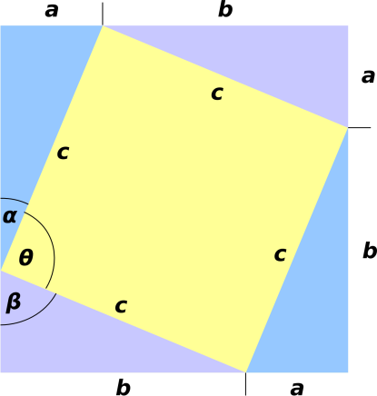 Figure 33
: Diagram for Proving the Pythagorean Theorem
Using the standard formula for the area of a triangle, the area of
each one of the bluish triangles is:
so the area of the four of them together is:
|
Area[4 triangles] | | = | | 2 a·b
|
| (64)
|
Using the standard formula for the area of a square, the area of the
entire colored area is:
|
Area[entire] | | = | | (a+b)2 |
| | | = | | a2 + 2 a·b + b2 |
| (65)
|
where we have expanded (a+b)2 using the binomial theorem.
We can infer that the area of the yellow square is the area of the
whole figure minus the four triangles.
|
Area[yellow] | | = | | a2 + 2 a·b + b2 − 2 a·b |
| | | = | | a2 + b2 |
| (66)
|
Meanwhile, we have another way of calculating the area of the yellow
square: It is just a square, with edges of length c:
Combining the two previous equations, we find
which is what we set out to prove.
To convert this outline into a real proof, we would have to go back
and fill in a bunch of details. For one thing, we would need to
assert that we are talking about figures in the flat, two-dimensional
plane. That’s important, because if you start drawing large triangles
on the surface of the earth, or any other space with intrinsic
curvature, the Pythagorean theorem is not valid. It’s bad luck to
prove things that aren’t true.
We also need to prove that the yellow region is in fact a square.
Just because we drew the diagram so as to make it “look” like a
square doesn’t count. In fact we can prove this, by using two facts
from Euclidean geometry: The interior angles of any triangle always
add up to 180∘. Therefore we know
We also know that the three angles α, β, and θ
add up to make a straight angle, so
Comparing this to the previous equation suffices to prove that θ
= 90∘. We also know that all four sides of the yellow area are
the same length. This suffices to prove that it is a square.
10.2 Discussion
The proof given here is similar to the one given by Pythagoras himself
in the mid-500s BC, except that ours is simpler. It is simpler
because we used algebra as well as geometry. Pythagoras didn’t have
algebra, so he needed an analog, graphical way of performing the
required subtraction.
Some algebraic ideas can be traced back 2000 years, but for most of
that time algebra was not very widely used. People used geometrical
constructions instead. Galileo, writing in the early 1600s, never
wrote an equals-sign in his entire life, as far as we can tell. Even
Newton, several decades later, even after he had invented calculus,
wrote books that largely avoided algebra. Often he would discover
things using algebra and calculus, and then reformulate them using
geometrical arguments alone. Obviously Newton understood algebra, but
in those days many people who were reading Newton’s books – even the
ones who were “aware” of algebra – did not trust it.
You can prove the Pythagorean theorem without using algebra,
but it is more work.
The Pythagorean theorem is so important the people have collected
several hundred different proofs.
11 The Square Root of 2 is Irrational
11.1 Preliminary Remarks
Elsewhere in this document, I have offered examples that have clear
practical applications. The example in this section – the
irrationality of √2 – is in a different category:
-
It has some large value to a small number of people.
- It has some small value to a large number of people. Small but nonzero.
I’m not going to pretend that the value is greater than it is.
|
Mathematicians are fascinated by this sort of thing. It says
something fundamental about numbers. It proves that there are more
kinds of numbers than you might have guessed.
|
|
For the other 99.9%
of the population, this topic is not nearly so fascinating. However,
it is interesting insofar as it shows you the sort of things that
mathematicians do.
|
|
Historians are also fascinated by this topic. Discovering
that √2 is irrational played a significant role in history,
including the history of science, philosophy, and even religion.
|
|
If
you are in the other 99.9% of the population, you should be very wary
whenever anybody tries to argue that something is important for
“historical” reasons. That reminds me too much of certain
“celebrities” who are “famous for being famous” even though they
have never accomplished anything of consequence.
|
|
|
|
You should also be very wary of lessons that claim to teach
a valuable skill while applying the skill to bogus problems.
Scoundrels have been using such claims for centuries, to justify
teaching stuff that wasn’t really all that important. The counter to
any such claim goes like this: If the skill is so valuable and broadly
applicable, why not show us some applications to real-world problems?
|
|
On the third hand, you don’t want to go overboard in the
direction of real applications, because sometimes the real-world
problems are unduly complicated, and some pedagogical simplification
is necessary. This is especially true in introductory algebra,
because so many of the applications involve using algebra in the
service of geometry in the service of physics in the service of
engineering, and those other subjects aren’t taught until later.
|
|
Even if some simplification is required, there should still be some
visible connection to real-world problems.
|
|
|
|
You should also be very wary of any claims that the topic
has “entertainment” value because the result is weird and
surprising. That is an awfully geeky argument, and it’s almost never
true. It seems to suggest that if the subject were even more weird
and surprising it would be more entertaining, which I don’t think is
true. A good teacher should make the result seem natural, relevant,
non-weird, and non-paradoxical. Weird is easy. Entertaining is hard.
Useful is hard.
|
For more about the math, history, and value of this topic, see
section 11.3.
A rational number, by definition, can be expressed as the ratio
of two integers; that is, one integer divided by another.
- 1/2 is rational.
- 8/6 is rational. We are not obliged to write the ratio in
lowest terms (although we always have the option to do so).
- 1.2345 is rational, because it is equal (by definition) to 12345/10000.
- 13 is rational, because it is equal to 13/1. The set of integers
is a subset of the set of rationals.
- 707/500 is a rational number that is approximately
equal to the square root of 2, but not exactly.
Now consider the number √2. Let’s call it S for short. We
know that S2 = 2. The question is, is S a rational number?
If S is rational, then all the following indented statements
are true:
S must be equal to A/B, for some integers A and B.
This is required, by the definition of rational number.
As a warm-up exercise, consider the fact that A must be either
even or odd, and similarly B must be either even or odd. If
they are both even, then A/2 is an integer and B/2 is an
integer and
In fact, we can go even further than that. There are
extremely efficient methods of calculating the greatest
common divisor of A and B. (Specifically, we could
use the Euclidean algorithm.) In any case, there exists
some integer G that is the greatest common divisor
of A and B. Therefore we can write:
where either the numerator or the denominator (or perhaps both) is
an odd number. So let’s define C and D, which we can use to
express S in lowest terms.
We can make progress by squaring the last expression:
Since the LHS is an even number, the RHS must be an even number.
That means C has to be an even number.
We can introduce a new number:
and we know that E must be an integer, not a half-integer,
because we have already proved that C must be even.
We can make further progress by considering the reciprocal of S.
Note that
as you can verify (perhaps by multiplying both sides by S). We
also know the following:
|
S | | = | | |
| S/2 | | = | | |
| | | = | | |
| | | = | | 1/S |
| S | | = | | |
| S2 | | = | | |
| 2 | | = | | |
| 2·E2 | | = | | D2 |
| (77)
|
which tells us that D must be even. This is very similar
to the way we proved that C was even.
To summarize, the only way we can have
S=C/D and 1/S=D/C is for both C and D to be even.
Now we have a real contradiction, because if both C and D are
even, that is inconsistent with the way we constructed them, when
we divided out the greatest common divisor of A and B.
To say the same thing more formally, if both C and D are even,
then 2G is a divisor of A and also a divisor of B, which is
inconsistent with the fact that G is (by construction) the
greatest common divisor of A and B. |
We can clarify the argument using a bit of Boolean algebra.
The structure of the argument so far is “P implies Q” where P
is the hypothesis that √2 is rational, and Q is all of the
indented statements collectively. You have to imagine that there is a
set of enormous parentheses around the indented stuff. There is a
distributive law in Boolean algebra, and if we were to carry out the
distribution, “P implies (X, Y, Z)” becomes “(P implies
X, P implies Y, P implies Z)”. That is to say, every
statement in the indented block must be true if √2 is rational
... but otherwise all bets are off.
The statement “P implies Q” means that whenever P is true then
Q must be true. We can check all four possible values of P and
Q, to see which of them are consistent with the proposition that P
implies Q.
|
| | P | | Q | | P implies Q ? |
|
| 0 | | 0 | | consistent |
| 0 | | 1 | | consistent |
| 1 | | 0 | | violated |
| 1 | | 1 | | consistent |
|
(78) |
Looking at the table, we see another way of summarizing what it means
to say “P implies Q”. It means that either Q is true or P
is false.
Consider the hypothesis that √2 is rational. This hypothesis
implies things that cannot be true. Therefore the hypothesis itself
must be false. In other words, √2 must be an irrational
number.
11.3 Discussion
Irrational numbers are not rare. If you take the square root of every
integer from 1 to a million, 99.9% of them will be irrational. In
fact, it can be proved that irrational numbers are infinitely more
numerous than rational numbers. That makes it somewhat ironic
that rational numbers were discovered first.
As mentioned in section 11.1, this proof has large
value to a small number of people, plus some small value to a large
number of people. I am not going to pretend the value is greater than
it is.
|
Proving that √2 is irrational is not high on the list
of practical real-world problems, in the sense that it won’t put
food on the table.
|
|
Just as an artist takes pride in his
craftsmanship, you can take pride in being able to represent √2
exactly.
|
|
Your calculator will tell you that √2 = 1.41421356237
or thereabouts, which is approximately true.
|
|
The decimal
representation cannot possibly be exactly true, because any decimal is
(by definition) a rational number.
|
|
The decimal approximation is good enough for a wide range of
practical purposes.
|
|
There are situations where approximating
√2 by a thirteen-digit-long decimal is not good enough. Such
situations are rather rare, but they do exist. In such a situation
the solution is usually not to use more digits; the smart solution is
to use algebra to restructure the problem so that you can more easily
calculate something that makes sense.
|
|
Sometimes people do things for strictly utilitarian
purposes.
|
|
Sometimes they do things for religious reasons. Sometimes
they do things for entertainment.
|
|
You could live to a ripe old age without being able to
prove that √2 is irrational.
|
|
Boolean algebra is
tremendously useful. It is worth learning, even if you never apply it
to √2. At some level, essentially everything that goes on in a
computer involves Boolean algebra. Also, the style of proof used here
can be used to prove other things. This style of proof is called
proof by contradiction.
|
The ancient Greeks who discovered that √2 was irrational
assigned religious significance to the discovery. They were not
expecting it to be irrational. They did not want it to be
irrational. They more-or-less worshipped numbers. It was a
combination of mysticism and mathematics. To them, integers were
perfect. It was a godlike perfection. One could even say that
integers are more perfect than the ancient Greek deities, who
were powerful but given to all sorts of bickering, thieving, adultery,
murder, et cetera.
They also knew about rational numbers. They had noticed the
connection between numbers and music, and were mightily impressed by
it. According to simple theory, an octave is a factor of 2/1, a perfect
fifth is a factor of 3/2, a perfect fourth is a factor of 4/3, et
cetera. In the real world, this theory does not entirely fit the
facts, but the ancient Greeks didn’t know that, and they overestimated
the importance of the theory.
Before √2 came along, the only numbers the ancient Greeks knew
about were rational numbers. The idea of something that was evidently
a number but outside their number system came as a real shock.
On the other hand, it reinforced their belief in the power of
mathematics. The idea that you can prove something to be true,
absolutely positively provably true, even though you didn’t expect it
to be true or want it to be true – that’s a really powerful idea.
This is proof far beyond the standard of “proof” that lawyers use in
court. This is not proof by the preponderance of the evidence. This
is not proof beyond a reasonable doubt. This is a mathematical proof,
and if you do it right, there is no wiggle room whatsoever.
There is also some value in understanding the proof, even if you don’t
place much value on the result. We proved something that you might
have thought was difficult or impossible to prove. It is proverbially
difficult to prove a negative, but that is exactly what we have done.
Also note that there are infinitely many rationals. Indeed there are
infinitely many rationals that are “close” to √2. Proving
that none of these is exactly equal to √2 requires some
seriously powerful tools.
Mathematics is telling you a negative message and also some positive
messages. It is telling you there are some things you simply cannot
do, such as describing the diagonal of a unit square in terms of an
exact rational number. On the positive side, mathematics is giving
you a glimpse of a whole new world, a new kind of numbers that you
never dreamed of. Another positive message is that the rules of
algebra – add subtract multiply divide associative distributive et
cetera – apply just fine to irrational numbers, just the same as
rational numbers, so you will very soon feel “at home” in this new
world.
It could be argued that this proof has value as a signpost at the
beginning of a long road. It tells you where to start. It puts you
on notice that there are other types of mathematical quantities out
there, not just integers and rational numbers.
On the other hand, one should not take the previous paragraph too
seriously. There are lots of other things that would serve equally
well as signposts, while having more direct practical applications.
Vectors, for example.
There are lots of things in this world that are fancier than
irrational numbers, such as transcendental numbers, complex numbers,
vector algebra, Clifford algebra, probability, calculus, topology, et
cetera. These things are tremendously useful. For example, if you
tried to do physics without vectors, it would be horrifically clumsy.
Doing quantum mechanics without complex numbers (or the equivalent)
would be impossible.
12 Tools and Techniques
12.1 Formalism, Notation, and Terminology
Ideas are primary and fundamental. Terminology is tertiary.
Terminology is important only insofar as it helps us formulate and
communicate the ideas. Conversely, if you find that the terminology
is causing problems, change the terminology.
It is almost never worth arguing about terminology. If you don’t
like the standard terminology, invent something better.
Einstein said that any theory should be as simple as possible, but not
simplier. John Reppy said that an experimentalist should never build
any more apparatus than necessary, or any less. The same goes for
mathematical formalism: It is usually a waste of time to build any
more formalism than necessary, or any less.
Formalism, notation, and terminology are tools. Sometimes they are
very helpful or even necessary ... but they are rarely an end unto
themselves.
12.2 Shortcuts
Math in particular, and science in general, can be considered a
collection of tools for solving problems, for reasoning about stuff,
and for avoiding mistakes.
Nobody really cares how much you work or how hard you work; mainly
they care how much you get done. By using the proper tools, you can
do the job faster and better.
Please do not think that all shortcuts are good, or all shortcuts are
bad. There are lots of possibilities:
- Some shortcuts fall into the “good tools” category,
producing superior results quickly.
- Some shortcuts fall into the “dirty tricks” category,
producing inferior results quickly.
- Some shortcuts fall into the “booby trap” category, wasting
time and effort, and producing bad results.
I am reminded of a story told by the Car Talk guys (reference 18), the story of The story of Delbert Joyner:
... who when asked to carry in a load of firewood by his grandfather,
tried to load 20 pieces in his arms
and walk from the woodpile to the house
and in doing so managed at one time or another
to drop each one of the 20 pieces
and when he finally reached the house after the half hour odyssey
the grandfather said y’know, you could have carried a few pieces
at a time and it is the lazy man who works the hardest.
That’s an amusing story, but the conclusion is misstated. A more
nuanced view is required.
- Trying to carry too much is a booby trap. It is the booby who
works hardest. A booby might have to work hard all day just to
survive.
- The skillful person has a choice: He might choose to work just
has hard as the other guy, but at the end of the day he has a lot more
to show for it. Alternatively, the skillful person might choose to
work somewhat less hard, and still have plenty to show for it, more
than enough to surive.
12.3 Abstraction
Sometimes making something more abstract makes it more useful.
Consider for example the number 12. Without being specific as to what
the questions are, imagine that the answers are as follows:
- The answer to question A is 12 pebbles.
- The answer to question B is 12 pencils.
- The answer to question C is 12 fish.
- The answer to question D is 12 dollars.
- The answer to question E is 12 apples.
- The answer to question F is 12 oranges.
- et cetera.
The number 12, by itself, is highly abstract. It is not the complete
answer to any of the aforementioned questions. However, it is
part of the answer to each of those questions, and unimaginably
many other questions. The fact that it is abstract makes it more
widely useful.
12.4 Symbolism
People are naturally good at symbolism. It’s the nature of the beast.
A two-year-old child playing with a baby doll knows it’s not a real
baby; it’s just a symbol representing a baby.
Spoken and written words are also symbols. The word “cat” sometime
serves to represent an actual cat. The word “felidae” serves to
represent something quite abstract, namely the phylogenetic family of
cat-like creatures, including lions, tigers, house-cats, et cetera.
We use numerals to represent numbers. For each number, there are many
ways of representing it. The following numerals all represent the
same number: twelve, 12, 12.000, 0xC, XII,
δώδєκα, et cetera.
13 Appendix – Miscellaneous Details
13.1 Sudoku Solution
13.2 Electronics Formulas in Gory Detail
| It must be emphasized that writing down all the
combinations and permutations like this is exactly what you are
NOT supposed to do. The smart thing would be to remember the
most fundamental equations and whatever others you use frequently –
plus the rules of algebra – and derive everything else if-and-when
needed. You could work for years as an electrical engineer without
ever writing things out in this level of mind-numbing
detail. |
We start with the 12 ways of combining and rearranging
Ohm’s law and the Joule heating law, using the four variables V,
I, R, and P.
If we define one more variable, the conductance, we get 12 more
equations:
| Again: writing down all the combinations and
permutations like this is exactly what you are NOT supposed to
do. The smart thing would be to remember the most fundamental
equations and whatever others you use frequently – plus the rules of
algebra – and derive everything else if-and-when needed. |
14 References
-
-
“XYZ Affair”
http://www.monticello.org/site/research-and-collections/xyz-affair -
John Denker,
“Learning, Remembering, and Thinking”
www.av8n.com/physics/thinking.htm -
John Denker
“Problem-Solving Checklist”
www.av8n.com/physics/problem-solving-checklist.htm -
David E. Joyce,
An annotated exposition of Euclid’s Elements,
http://aleph0.clarku.edu/~djoyce/java/elements/An example of a missing postulate is given at:
http://aleph0.clarku.edu/~djoyce/java/elements/bookI/propI4.html
-
Insofern sich die Sätze der Mathematik auf
die Wirklichkeit beziehen, sind sie nicht sicher, und insofern sie
sicher sint, beziehen sie sich nicht auf die Wirklichkeit.
Albert Einstein,
“Geometrie und Erfahrung”
English Translation: “Geometry and Experience”
Lecture to the Prussian Academy of Science (27 January 1921).
http://quod.lib.umich.edu/u/umhistmath/ABR1192.0001.001/
http://www-history.mcs.st-and.ac.uk/Extras/Einstein_geometry.html
http://pascal.iseg.utl.pt/~ncrato/Math/Einstein.htm
-
Jessica Lahey
“Teaching Math to People Who Think They Hate It”
http://www.theatlantic.com/education/archive/2014/10/teaching-math-to-people-who-think-they-hate-it/381125/2/ -
Volker Ecke and Christine von Renesse
with Julian F. Fleron and Philip K. Hotchkiss,
Discovering the Art of Mathematics: Games and Puzzles
https://www.artofmathematics.org/sites/default/files/books/games-2013-06-06.pdf
(The whole book is available online, free for all.) -
John Denker,
“Ruler-Drop Measurement of Reaction Time”
www.av8n.com/physics/ruler-drop.htm -
John Denker,
“spreadsheet for calculating hybrid car economy”
./economy-hybrid-car.xls
-
John Denker,
“Hints on How to Do Math”
www.av8n.com/physics/math-hints.htm -
John Denker,
“Scaling Laws”
www.av8n.com/physics/scaling.htm -
Joint Committee for Guides in Metrology
“International Vocabulary of Metrology –
Basic and General Concepts and Associated Terms (VIM)”
http://www.nist.gov/pml/div688/grp40/upload/International-Vocabulary-of-Metrology.pdf -
Douglas Isbell, Mary Hardin, Joan Underwood,
“MARS CLIMATE ORBITER TEAM FINDS LIKELY CAUSE OF LOSS”
http://mars.jpl.nasa.gov/msp98/news/mco990930.html -
“Mars Climate Orbiter Fact Sheet”
http://mars.jpl.nasa.gov/msp98/orbiter/fact.html -
John Denker,
“spreadsheet for calculating linear and quadratic examples”
./algebra-examples.xls
-
John Denker,
“Cause and Effect”
www.av8n.com/physics/causation.htm -
John Denker,
“The Spiral Approach to Thinking and Learning”
www.av8n.com/physics/spiral-approach.htm -
“Car Talk” episode 1514 segment 3
“The Stingy Man Spends the Most”
http://www.cartalk.com/content/1514-stingy-man-spends-most