Hints on How to Do Math
John Denker
* Contents
1 Fundamental Suggestions
Here are some hints on how to do basic math calculations.
These suggestions are intended to make your life easier. Some of them
may seem like extra work, but really they cause you less work in the
long run.
This is a preliminary document, i.e. a work in progress.
-
- 1.
Be tidy and systematic. Whenever you have data in tables,
especially when place-value is important, be sure to keep things
lined up in neat columns and neat rows. See section 4 for
an example of how this works in practice.
- 2.
If your columns are wobbly, get a pad of graph
paper and see if that helps. If you don’t have a supply of
store-bought graph paper, you can make graph paper on your computer
printer. There are freeware programs that do a very nice job of
this.
If that’s too much bother, start with a plain piece of paper and
sketch in faint guidelines when necessary.
- 3.
Paper is cheap. If you find that you are
running out of room on this sheet of paper, get another sheet of
paper, rather than squeezing the calculation into a smaller space.
See section 4 for an example of using extra paper to
achieve a better result.
- 4.
The whole calculation should be structured as a succession
of true statements. The first statement is true, the next statement
is true, and the statement after that, et cetera. Each statement is
a consequence of the previous statements (in conjunction with known
theorems, and the “givens” of the problem). Finally, we get to the
bottom line, and we know it is true. An example of this can be seen
in reference 1.
- 5.
Sometimes, especially for long and/or complex calculations, it
helps to organize your calculation in two columns. An example of
this can be seen in reference 1. In the left column, you
write an equation. In the right column, make a note as to how you
derived that equation. (Numbering all your equations makes this
easier.) If there isn’t enough width to do this easily, turn the
paper 90 degrees, so it becomes wider and less tall. (Writing paper
isn’t suitable for this, so use graph paper ... or lacking that,
plain white paper.)
- 6.
Avoid writing down an un-named number like 17, or an
un-named expression like a+17 ... because you might forget the
meaning thereof. Instead, whenever possible, write down an
equation such as b=a+17. That way you can point to every
item on the page and say that’s true, that’s true, that’s true... in
accordance with the strategy described in item 4.
- 7.
If the meaning of variables such as a and b is not
obvious, write down a legend somewhere (like the legend of a map),
explaining in a sentence or two the meaning of each variable. That
is, a name is not the same as an explanation. Do not expect the
structure of a name or symbol to tell you everything you need to
know. Most of what you need to know belongs in the legend. The name
or symbol should allow you to look up the explanation in the legend.
- 8.
You’re allowed to use multi-letter variable names.
For example, in a situation where you need F to stand for force
and F to stand for the Helmholtz free energy and F to stand
for the electromagnetic field bivector, just spell out what
you mean: Force = m a.
As mentioned in item 7, the name cannot encode every
interesting detail. However, it can at least be unique, so you can
look up the details.
- 9.
It is important to be able to go back and check the
correctness of the calculation you have done. See
section 4 and/or reference 1 for examples of
what this means in practice.
- 10.
As a corollary of item 9: Don’t perform
surgery on your equations. That is, once you write down a correct
equation, don’t start crossing out terms (or, worse, erasing terms)
and replacing them with other expressions. Such a substitution may
be “mathematically” correct, if the replacement is equal to the
thing being replaced ... but it is a bad strategy, because it makes
it hard for you to check your work. Instead, write a new equation.
Leave the old equation as it is. Paper is cheap. An example of this
can be seen in reference 1.
- 11.
Don’t change the meaning of variables.
The classic scenario is this: You start out having an expression for
y as a function of x. You solve for the inverse function, so now
x is known as a function of y. You want to plot the new
function, but for some reason you feel obliged to plot things in the
form y versus x, so you are tempted to reverse the meaning of the
variables.
This is one of the 77 habits of highly crazy people. Don’t do it!
Do not succumb to this temptation.
Don’t change horses in mid-stream.
Don’t change the meaning of x in mid-calculation.
|
|
|
|
Instead, you should set the whole calculation aside and start over
using variables that don’t need to be redefined. Using meaningful
(or at least mnemonic) variable names will help. For instance if you
started with current as a function of voltage, use the traditional
symbols I and V. You can plot I versus V just as easily as
V versus I, with no temptation to change the meaning. If you
really have no idea what the symbols mean, use non-committal names
such as p versus q. You can plot q versus p just as easily
as p versus q.
More generally, introductory textbooks tend to fall
into the following habits:
- ☠ Supposedly, x is always the input and y is
always the output.
- ☠ Supposedly, on a graph, x is always horizontal
and y is always vertical
- ☠ Supposedly, on a graph, the input is always
horizontal and the output is always vertical.
In mathematics, none of those things is actually required. You
should break those habits. (Some spreadsheet apps force on you the
idea that the horizontal direction is called x and the vertical
direction is called y, but it is still a bad idea.)
- 12.
When you think of x on a graph, do not think in terms of
the x “axis”; see reference 2 for an explanation of this
issue.
- 13.
Keep track of the units for each expression. For example,
the statement “x=2.5 inches” means something rather different
from “x=2.5 meters” ... and if you shorthand it as “x=2.5”
you’re just asking for trouble.
Sometimes the penalty for getting this wrong is on the order of three
hundred million dollars, as in the case of the Mars Climate Orbiter
(reference 3).
 Figure 1
: Mars Climate Orbiter mission logo
./img48logo-98t-s.png
Most computer languages do not automatically keep track of the units,
so you will have to do it by hand, in the comments. If the
calculation is nicely structured, it may suffice to have a
legend somewhere, spelling out the units for each of the
variables. If variables are re-used and/or converted from one set of
units to another, you need more than just a legend; you will need
comments (possibly quite a lot of comments) to indicate what units
are being used at each point in the code.
One policy that is sometimes helpful (but sometimes risky) is to
convert everything to SI units as soon as it is read in, even in
fields where SI units are not customary. Then you can do the
calculation in SI units and convert back to conventional units (if
necessary) immediately before writing out the results. (This is
problematic when writing an “intermediate” file. Should it be SI
or customary? How do you know the difference between an
“intermediate” result and a final result?)
It is certainly possible for computer programs to keep track of the
units automatically. A nice example is reference 4. It is
a shame that such features are not more widely available
- 14.
The factor-label method is a convenient and
powerful way of converting units when necessary. The correctness of
this method is a direct consequence of the axioms of algebra, since
it starts by multiplying by unity, which is allowed by the axioms.
- 15.
Haste makes waste, especially with multi-step processes. If
you work methodically, you’ll get the right answer the first time,
and that’s all there is to the story. If you try to do it twice as
fast, you’ll get the wrong answer, and then you’ll have to do it over
again ... and again ... and again.
2 Multiple Methods of Solution
Here’s a classic example: The task is to add 198 plus 215. The
easiest way to solve this problem in your head is to rearrange it as
(215 + (200 − 2)) which is 415 − 2 which is 413. The small point
is that by rearranging it, a lot of carrying can be avoided.
One of the larger points is that it is important to have multiple
methods of solution. This and about ten other important points are
discussed in reference 5.
3 Drawing Inequalities
The classic "textbook" diagram of an inequality uses shading to
distinguish one half-plane from the other. This is nice and
attractive, and is particularly powerful when diagramming the
relationship between two or more inequalities, as shown in
figure 2.
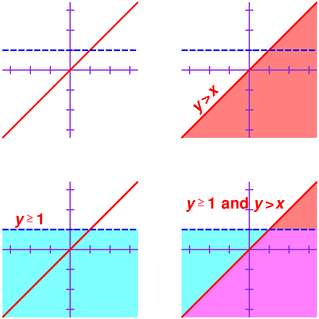 Figure 2
: Inequalities Represented using Shading
However, when you are working with pencil and paper, shading a
region is somewhere between horribly laborious and impossible.
It is much more practical to use hatching instead, as shown
in figure 3.
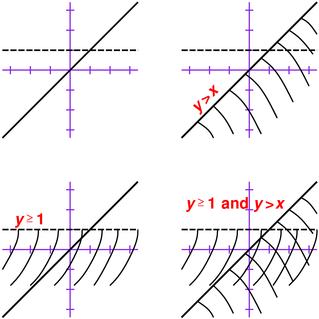 Figure 3
: Inequalities Represented using Hatching
Obviously the hatched depiction is not as beautiful as the shaded depiction,
but it is good enough. It is vastly preferable on cost/benefit
grounds, for most purposes.
Some refinements:
- I recommend hatching the excluded half-plane, so that the
solution-set remains unhatched rather than hatched. This is
particularly helpful when constructing the conjunction (logical
AND) of multiple inequalities.
- I recommend using solid lines versus dashed lines to distinguish
“≥” inequalities from “>” inequalities. If you’re going to
hatch the excluded half-plane, use solid lines for the “>”
inequalities, to show that the boundary itself is excluded.
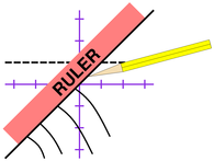
- As suggested in figure 4, for linear
inequalities you can do the hatching faster and more accurately with
the help of a ruler or straightedge, which makes it easy to ensure
that none of the hatches stray into the wrong region.
4 Long Multiplication
For most people, if all you want to do is multiply numbers, is
reasonable to just forget about long multiplication. You can use a
calculator for multiplying numbers. On the other hand, if you’re
interested in understanding how long multiplication works, here is
an explanation.
A video covering mostly the same ideas is in reference 6.
4.1 Background
Short multiplication refers to any multiplication problem that
consists of multiplying a one-digit number by another one-digit
number. That means everything from 0×0 through 9×9.
Long multiplication refers to multiplying multi-digit numbers. We are
about to discuss a highly efficient algorithm for doing this.
As a prerequisite for doing long multiplication, you need to be able
to do short multiplication reliably.
- Your short multiplication doesn’t have to be fast. Reliability
is more important than speed, so take your time.
- Your don’t need to have your short multiplication facts
fully committed to memory at this stage. If necessary,
write out a multiplication table and use that to help you
do the required short multiplications.
Speed will improve gradually over time. The short multiplication
facts will become consolidated in your memory over time. Indeed, long
multiplication gives you plenty of practice doing short
multiplication, so we can kill two birds with one stone.
4.2 Some Simple Examples
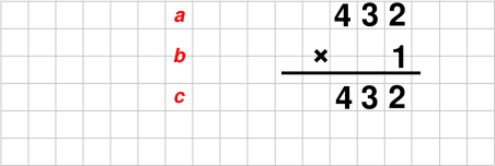
Let’s start by doing a super-simple example. Let’s multiply 432 by
1. You can do that in your head. The answer is written out in
figure 5, in the standard form used for long
multiplication problems.
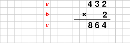
Multiplication by 2 is almost as easy, as shown in figure 6:
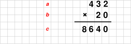
Multiplication by 20 is also easy; all we need to do is shift the
previous result over one place, as shown in figure 7:
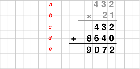
Here’s a more interesting example. Let’s multiply 432 by 21. We can
reduce the workload if we rewrite 21 as 20+1. We can express that as
an equation:
So now we are multiplying 4321×(20+1). The equation is:
There are two ways of understanding where equation 2 comes
from. One way is to start with equation 1 and multiply both sides
by 432. Another way is to start with the left-hand side of
equation 2 and replace the 21 by something that is equal to
it; in other words, to do a substitution.
We can apply the distributive law to the right-hand side
of equation 2. That gives us:
|
| |
432×21 | | = | | 432×(20+1) | |
(3a)
|
|
| |
| | = | | 432×20 + 432×1 | |
(3b)
|
|
Both of the multiplications in equation 3b are easy, and
indeed we have already done them. Plugging in the results of these
multiplications gives us:
|
| |
432×21 | | = | | 432×(20+1) | |
(4a)
|
|
| |
| | = | | 432×20 + 432×1 | |
(4b)
|
|
| |
| | = | | 8640 + 432 | |
(4c)
|
|
So at this point, there’s no more multiplying to be done. All that
remains is a simple addition problem, as shown in figure 8. The multiplication problem shown in gray is
exactly equivalent to the addition problem shown in black.
Note that we can get by without writing the zero at the end of line
d in the figure. The bottom-line result is the same, whether we
write this zero or not, provided we keep things properly lined up in
columns, as shown in figure 9. In the number
system we are using, the Hindu number system, we normally think of
zeros like this as being necessary to indicate place value. However,
that’s not strictly true. You don’t need to write the zeros, provided
you have some other way of keeping track of place value.
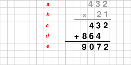 Figure 9
: Suppressing an Unnecessary Zero
You are allowed to write the zero (as in figure 8)
if that’s convenient, but you are also allowed to skip it (as in
figure 9) if that’s more convenient.
Long multiplication depends on lining stuff up in columns, as a way of
keeping track of place value. Therefore, when learning to do long
multiplication, use graph paper. This will help you keep things
properly lined up. Tidyness counts for a lot when doing long
multiplication.
After you’ve done hundreds of these things, and have learned to be
super-tidy, you can do without the graph paper, but until then you’ll
save yourself a lot of grief if you use graph paper. The best thing
is to get a lab book, which is a bound book containing blank graph
paper on every page. Such things are cheap and readily available from
office-supply stores. The second-best thing is to use graph paper in
pad form, or perhaps loose-leaf form. If you have a printer attached
to your computer, there are apps that will print graph paper for you,
in any imaginable style.
Use graph paper
at least at first.
|
|
|
|
Note that numbers tend to be taller than they are wide. For this
reason, rather than writing every row of numbers on the lines of the
graph paper, it looks nicer if each row of numbers is 1½ lines
below the previous one. You can see how this works in the figures in
this section.
The principle here is that the graph paper is supposed
to help you, not hobble you. If using the vertical lines is
helpful, use the vertical lines. If using the horizontal lines in
the obvious way is not optimal, use them in some less-obvious way.There are always lots of people trying to make you color inside the
lines, but any kind of originality, artistry, or creativity requires
coloring outside the lines. Math, if it’s done right, involves lots
of creativity. Don’t be afraid to color outside the lines.
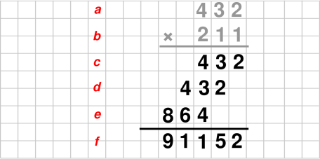
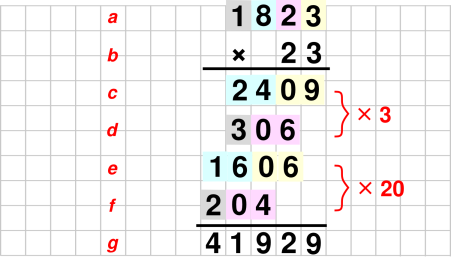
Let’s do one more example. Let’s multiply 432 by 211. We use the
same trick as before: We pick 211 apart, digit by digit. That is, we
write 211 = 200 + 10 + 1. Multiplying by 200 is easy; just multiply
by 2, and then shift the result two decimal places. The whole procedure
can be carried out very efficiently, if you organize it properly,
as shown in figure 10.
4.3 The Recipe
The recipe for doing long multiplication is based on simple ideas:
- Break the given factors down into their individual digits.
- Multiply everything on a digit-by-digit basis. This
requires doing a lot of short-multiplication problems.
- Add up all the products, with due regard for place value.
Long multiplication
= lots of short multiplications
+ addition
with place value.
|
|
|
|
We will mostly use the same approach as we used in
section 4.2. The only difference is that this time we
will need to pick apart both of the factors into their
individual digits. (Previously we only picked part the second
factor.)
As mentioned in section 4.2, the rationale for doing
things this way is based on the distributive law and the axioms of the
number system. This is discussed in more detail in section 4.7.
There is an easy and reliable method for arranging the calculations.
We illustrate the method using the question shown in figure 11.
The first step is to write down the question. It is important to line
up the numbers as shown, so that the ones’ place of the top number
lines up with the ones’ place of the bottom number, and so on for all
the other digits. Keeping things aligned in columns is crucial, since
the colums represent place value. As mentioned in item 1,
tidiness pays off.
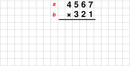 Figure 11
: Long Multiplication Example #1 – The Question
If one of the factors is longer than the other, it will usually
be more convenient to place the longer one on top. That’s not
mandatory, but it makes the calculation slightly more compact.
You may omit the multiplication sign (×) if it is obvious from
context that this is a multiplication problem (as opposed to an
addition problem).
We proceed digit by digit, starting with the rightmost digit in the
bottom factor, and proceeding systematically right-to-left. We do
things in order of increasing place value, right to left. That makes
sense, especially when doing additions, because a carry can affect the
next column (to the left), but never the previous column. This is
opposite to the direction of reading English text, which is
unfortunate, but there’ s nothing we can do about it.
So, let’s look at the rightmost digit in the bottom factor in our
example. It’s a 1. We multiply this digit into each digit of the
other factor, digit by digit, working systematically right-to-left
across the top factor.
We place these results in order in row c, with due regard for place
value. The 1×7 result goes in the ones’ place, the 1×6
result goes in the tens’ place, and the 1×5 result goes in the
hundreds’ place, and so forth, as shown in row c in figure 12. Actually, multiplication by 1 is so easy that you
can just copy the whole number 4567 into row c without thinking
about it very hard. So far, this is just like what we did in
section 4.2.
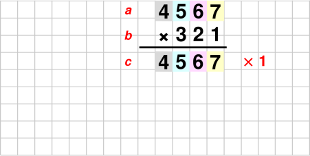 Figure 12
: Long Multiplication Example #1 – First Row
Note: You may wish to leave a little bit
of space above the numbers in row c, for reasons that will
become apparent later.Also note: In all the figures in this section, anything shown in
black is something you actually write down, whereas anything shown
in color is just commentary, put there to help us get through the
explanation the first time.
That is all we need to do with the low-order digit of the bottom
factor. We now move on to the next digit of the bottom factor. In
this case it is a 2.
At this point in this example, things get interesting, because some of
the short-multiplication results are two digits long. There is no
way to write all of them in a single row. Fortunately, we are allowed
to use multiple rows. One possibility is to spread things out as
shown in figure 13. We write 2×7=14 in row
d, and then write 2×6=12 on row e, and so on.
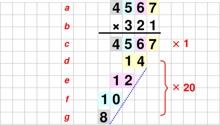 Figure 13
: Long Multiplication Example #1 – Spread-Out Form
It is theoretically possible to write the product 4567×2 on a
single row, but this would require doing a bunch of additions, but we
choose not to do that. We are going to do all the short
multiplications first, and then do all the additions later. This
requires slightly more paper, but it is vastly easier to do, easier to
understand, and easier to check.
As previously mentioned, the procedure is to pick a digit from the
lower factor, and multiply this digit into each digit of the upper
factor. The result of the first such multiplication is 2×7=14,
which we place in row d. Alignment is crucial here. The 14 must be
aligned under the 2 as shown. That’s because it “inherits” the
place value of the 2.
Next we multiply 2×6=12. You might be tempted to write this in
row d, but there is no room for it there, so it must go on row e,
as shown in the figure. Again alignment is critical. This product is
shifted one place to the left of the previous product, because it
inherits additional place value. It inherits some from the 2 (in the
bottom factor) and some from the 6 (in the top factor). Since we are
working systematically right-to-left, you don’t need to think about
this too hard; just remember that each of these short-division
products must be shifted one place to the left of the previous one, as
suggested by the diagonal dotted blue line in
figure 13.
Let me explain the color-coded backgrounds. In row d, the 14 has a
yellow background, because it is derived from the 7 in row a, which
has a yellow background. Similarly the 12 in row e yas a pink
background, because it is derived from the 6 in row a, which has a
pink background.
Although figure 13 is good for illustrating the
principles involved, it is unnecessarily spread out. It would be
better to write things more compactly, as shown in figure 14, because this makes it easier to keep things properly
aligned. (The objective here is not to save paper. Remember, paper
is cheap, and trying to save paper is almost always a bad idea.
The advantage of the compact representation is that it makes it
easier to keep things lined up in columns.)
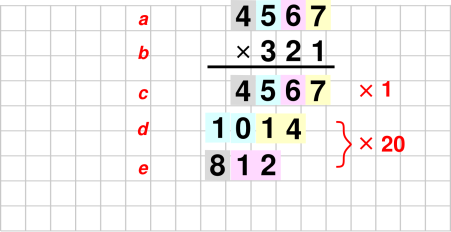 Figure 14
: Long Multiplication Example #1 – Compact Form
Note the pattern of placing successive short-division results on
alternating rows. There is guaranteed to be enough room to do this,
because the product of two one-digit numbers can never have more than
two digits.
We are now more than half-way finished.
At this point (or perhaps earlier), if you are not using grid-ruled
paper, you should lightly sketch in some vertical guide lines. The
tableau has become large enough that there is some risk of messing up
the alignment, i.e. putting things into the wrong columns, if you
don’t put in guide lines.
That’s all for the “2” digit in the bottom factor. We now proceed
to the “3” digit. We multiply this by each of the digits in the top
factor, in the now-familiar fashion. All the short-multiplication
results from this step are put in rows f and g.
At this point, all of the short multiplications are complete. In
figure 15, you can see where everything comes from.
The color-coded background indicates which digit of the upper
factor was involved, and the row indicates which digit of the
bottom factor was involved.
 Figure 15
: Long Multiplication – Penultimate
Stage
All that remains is a big addition problem, adding up rows c through
g inclusive. Draw a line under row g as shown in figure 16, and start adding.
- You can use the space above row c to keep track of carries if
you wish
- On the other hand, writing the carries is not mandatory. There
are never very many carries, and you don’t need to remember them for
very long, so keeping track of them is easy, no matter how you do it.
Personally, I prefer not writing the carries. That’s because
whenever I’m adding a tall column of numbers, I do it twice: once from
top to bottom, and once from bottom to top. This is a good way to
double-check the results. When adding bottom-to-top, the carry gets
added at the bottom, and having it written at the top creates more
problems than it solves. Figure 17 shows an example of
addition with unwritten carries.
In any case, the result of the big addition is the result of the
overall multiplication problem, as shown on row h of figure 16.
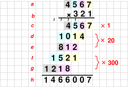 Figure 16
: Long Multiplication – Final Result
4.4 Keeping Things Properly Lined Up
Let’s be super-explicit about the rules for keeping things lined up in
columns.
It pays to think of the short-multiplication products in groups.
The groups are labeled in figure 16. Row c is the “by
one” group. Rows d and e form the “by twenty” group. Rows f
and g form the “by three hundred” group.
The first rule is that each group is shifted over one place relative
to the group above it. For example, the rightmost digit in row d is
shifted one place relative to the rightmost digit on row c.
Similarly, the rightmost digit in row f is shifted one place
relative to the rightmost digit in row d.
This rule has a simple explanation: The groups inherit place value
from the digit in the lower factor that gave rise to the group.
As another way of expressing the same rule: Each group is lined up
under the digit in the lower factor that gave rise to the group. For
example, in figure 16, the group on lines f and g is
lined up under the 3 in the lower factor. Similarly, the 8 on line
e is shifted over one place relative to the 10 on line d.
The second rule is that within each group, each short-multiplication
product is shifted over one place relative to the previous factor in
the group. For example, in figure 16, the 12 on line e
is shifted over one place relative to the 14 on line d.
This rule also has a simple explanation: Each of the products inherits
some place value from the digit in the upper factor that gave rise to
the product.
4.5 Another Example
Let’s do another example, as shown in figure 17, which
illustrates one more wrinkle.
This example calls attention to the situation where some of the
short-multiplication products have one digit, while others have two.
You can see this on row c of the figure, where we have 3×3=9
and 3×8=24. In most cases it is safer to pretend they all have
two digits, which is what we have done in the figure, writing 9 as 09.
Similarly on line d we write 6 as 06. This makes the work fall into
a nice consistent pattern. It helps you keep things lined up, and
makes the work easier to check.
In some cases, such as 345×1 or 432×2,
all the short-multiplication products have one digit, so you can
write them all on a single line, if you wish. This is less work,
and more compact. On the other hand, remember the advice in
item 3: paper is cheap. You may find it helpful to
write the short-multiplication products as two digits even if you
don’t have to.If even one of the products (other then the leftmost one) requires
two digits, you will almost certainly need two rows anyway, so you
might as well get in the habit of using two rows.
Mathematically speaking, writing one-digit products as two digits is
unconventional, but it is entirely correct. It has the advantage of
making the algorithm more systematic, and therefore easier to check.
In any case, the result of the addition is the result of the overall
multiplication problem, as shown on row g of figure 17.
That’s all there is to it.
4.6 Discussion
This algorithm ordinarily uses two rows of intermediate results for
each digit in the bottom factor. In special cases, we can get by with
a single row.
Another hallmark of this algorithm is that we first do all the short
multiplying, and then do all of the adding. Every time we do a short
multiplication, we just write down the answer. This has several major
advantages:
- It makes the short multiplications go faster. When you are
multiplying, you are just multiplying. You don’t need to worry about
adding. There are no carries to keep track of.
- There are fewer things to go wrong.
- It makes it easy to check your work. You can re-do each of the
multiplications and check to see that you get the same answer.
Conversely, if any of the short-multiplication results looks
suspicious, you can easily figure out where it came from, and
re-check the multiplication.
This differs from the old-fashioned “textbook” approach, which uses
only one row per digit, as shown below. The old-fashioned approach
supposedly uses less paper – but the advantage is slight at best, and
if you allow room keeping track of “carries” throughout the tableau,
the advantage becomes even more dubious. Besides, paper is cheap, so
it is penny-wise and pound-foolish to save paper at the cost of making
the algorithm more complex, more laborious, and less reliable.
The old-fashioned approach may look more compact, but it involves more
work. You have to do the same number of short multiplications, and a
greater number of additions. It requires you to do additions
(including carries) as you go along.
Last but not least, it makes it much harder to check your work.
| | | | 4 | 5 | 6 | 7 |
| | | × | | 3 | 2 | 1 |
|
| | | | 4 | 5 | 6 | 7 |
| | | 9 | 1 | 3 | 4 | |
| 1 | 3 | 7 | 0 | 1 | | |
|
| 1 | 4 | 6 | 6 | 0 | 0 | 7
|
The old-fashioned approach.
Not recommended.
Remember, paper is cheap (item 3) and it is important
to be able to check your work (item 9).
4.7 Conceptual Foundation
The long-multiplication algorithm as presented here is guaranteed to
work. That’s because it is quite directly based on the fundamental
axioms of arithmetic, including the axioms of the number system.
Consider the numbers 4567 and 321 which appeared in section 4.3. We can expand 4567 as 4000+500+60+7. That’s what
4567 means, according to the rules of the Hindu number system.
Similarly, we can expand 321 as 300+20+1.
The reason for expanding things this way is that in the sum
4000+500+60+7, each term consists of a single non-zero digit, with
some place value.
The next step is to expand the product 4567×321 as
(4000+500+60+7)×(300+20+1). We can then carry out the product
in the expanded form, term by term, by repeated application of the
distributive law. In our example, there are four terms in the first
factor and three terms in the second factor, which give us 12 terms in
the product, as shown in table 1. Each term in
the product consists of a single-digit multiplication – a short
multiplication – with some place value.
| | | 300 | | 20 | | 1 |
| 7: | | 2100 | | 140 | | 7 |
| 60: | | 18000 | | 1200 | | 60 |
| 500: | | 150000 | | 10000 | | 500 |
| 4000: | | 1200000 | | 80000 | | 4000 |
Table 1: Long Multiplication, Expanded
So, the main thing the algorithm needs to do is to help you write down
these 12 numbers in a convenient, systematic way.
One convenience is that the algorithm saves you from writing down all
those zeros. You pay a small price for this. The price is that you
absolutely must keep the numbers properly lines up in columns.
The rules about how to write the numbers in columns are not magic;
they are just a way of keeping track of place value. They are a
direct consequence of the axioms of arithmetic, including the
axioms of the number system.
In particular, the “12” that appears in the lower-left element of
table 1 is the same “12” that appears at the
left of row g in figure 16 ... and the latter is lined
up in columns so as to give it the correct place value.
4.8 Terminology: Product, Factor, Multiplier, and Multiplicand
The word “multiplicand” is more-or-less Latin for “the thing being
multiplied”.
In figure 11, some people insist that the top number
should be called the “multiplier” and the bottom number should be
called the “multiplicand”. Meanwhile, other people insist on
naming them the other way around. Quite commonly, they use the words
in ways inconsistent with the supposed definition.
All of this is nonsense. Multiplication is commutative. Pretending
to see a distinction between the two numbers is the silliest thing
since the holy war between the Big-Endians and the Little-Endians.
Furthermore, multiplication is associative, so we could easily have
three or more things being multiplied, as in
12×32×65×99, in which case it is obviously hopeless
to attempt to distinguish “the” multiplier from “the”
multiplicand.
The modern practice is to call both of the numbers in figure 11 the factors. You can equally well call both of
them multipliers, or call both of them multiplicands. Along the same
lines, modern practice is to say that an expression such as
12×32×65×99 is a product of four factors.
4.9 Terminology: Times versus Multiplied By
There are also holy wars as to whether 4567×321 means 4567
“times” 321, or 4567 “multiplied by” 321. The distinction is
meaningless. Don’t worry about it.
5 Long Division
The usual “textbook” instructions for how to do long division are
both unnecessarily laborious and unnecessarily hard to understand.
There’s another way to organize the calculation that is much less
mysterious and much less laborious (especially when long multi-digit
numbers are involved).
Note that as discussed above, keeping things lined up in columns
is critical. It may help to use grid-ruled paper, or at least to
sketch in some guidelines.
A video covering mostly the same ideas is in reference 7.
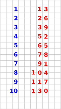
5.1 The Algorithm : Using a Crib
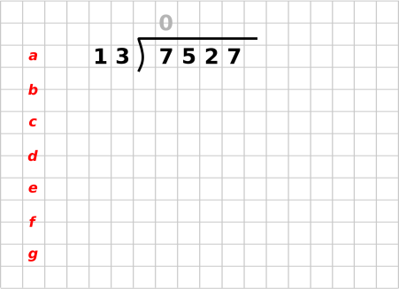
Suppose the assignment is to divide 7527 by 13. After writing down
the statement of the problem, and before doing any actual dividing, it
helps to make a crib, as shown in figure 18.
This is just a multiplication table, showing all multiples of the
assigned divisor, which is 13 in our example.
It is super-easy to construct such a table, since no multiplication is
required. Successive addition will do the job. We need all the
multiples from ×1 to ×9, but you might as well calculate
the ×10 row, by adding 117+13. This serves as a valuable
check on all the additions that have gone before.
We now begin the main part of the algorithm. The first step is to
consider the leading digit of the dividend (which in this case is a
7). This is less than the divisor (13). There is no way we can
subtract any nonzero multiple of 13 from 7. Therefore we leave a
blank space above the 7 and proceed to the next digit. We could
equally write a zero above the 7, as shown in gray in figure 20, but that’s just extra work and confers no lasting
advantage, since leading zeros are meaningless.
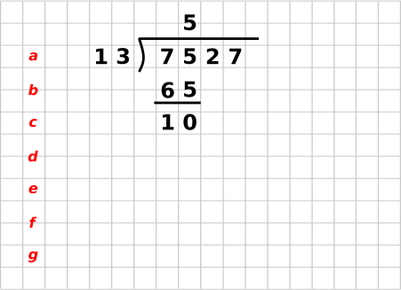
Now consider the first two digits together, namely the 7 and the 5.
Look at the crib to find the largest entry less than or equal to 75.
It is 65, as in 5×13=65. Copy this entry to the appropriate
row of the division problem, namely row b. Align it with the 75 on
the previous row. Since this is 5 times the divisor, write a 5
on the answer line, aligned with the 75 and the 65, as shown. Check
the work, to see that 5 (on the answer line) times 13 (the divisor, on
line a), equals 65 (on line b).
Now do the subtraction, namely 75−65=10, and write the result
on line c as shown.
When we take place value into account, the 5 in the quotient is short
for 500, and the 65 that we just subtracted is short for 6500.
Normally we would need to write the zeros explicitly as part of these
numbers, to indicate place value. However, in this situation we are
using columns to keep track of place value. If we keep everything
properly lined up, we don’t need to write the zeros. In fact, the
zeros would just get in the way (especially in the quotient) so we are
better off not writing them.
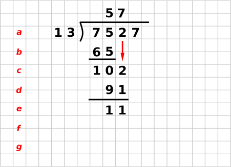
We now shift attention to the situation shown in figure 21. Bring down the 2 from the dividend, as shown by the
red arrow. So now the number we are working on is 102, on line c.
The steps from now on are a repeat of earlier steps.
Look at the crib to find the largest entry less than or equal to 102.
It is 91, as in 7×13=91. Write copy this entry to the division
problem, on row d, directly under the 102. Since this came from row
7 of the crib, write a 7 on the answer line, aligned with the 102 and
the 91, as shown. Check the work, to see that 7 (on the answer line)
times 13 (the divisor, on line a), equals 91 (on line d). Do the
subtraction.
As a check on the work, when doing this subtraction,
the result should never be less than zero, and should never be
greater than or equal to the divisor. Otherwise you’ve used the
wrong line from the crib, or made an arithmetic error.
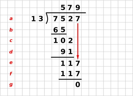
We now shift attention to the situation shown in figure 22. Bring down the 7, look in the crib to find the
largest entry less than or equal to 117, which is in fact 117, as in
9×13=117. Since this came from line 9 of the crib, write a 9
on the answer line, properly aligned.
The final subtraction yields the remainder on line g. The remainder is
zero in this example, because 13 divides 7527 evenly.
5.2 Remarks
The crib plays several important roles.
Perhaps the crib’s most important advantage, especially when people
are first learning long division, is that the crib removes the mystery
and the guesswork from the long division process. This is in contrast
to the “trial” method, where you have to guess a quotient digit, and
you might guess wrong. Using the crib means we never need to do a
short division or trial division; all we need to do is skim the table
to find the desired row.
We have replaced trial division by multiplication and table-lookup.
Actually we didn’t even need to do any multiplication, so it would be
better to say we have replaced trial division by addition.
Another advantage is efficiency, especially when the dividend has many
digits. That’s because you only need to construct the crib once (for
any given divisor), but then you get to use it again and again, once
for each digit if the dividend. For long dividends, this saves a
tremendous amount of work. (This is not a good selling point
when kids are just learning long division, because they are afraid
of big multi-digit dividends.) Setting up the crib is so fast that
you’ve got almost nothing to lose, even for small dividends.
Another advantage is that it is easy to check the correctness of the
crib. It’s just sitting there begging to be checked.
When bringing down a digit, you may optionally bring
down all the digits. For instance, in figure 21, if you bring down all the digits you get 1027 on
row c. One advantage is that 1027 is a meaningful number, formed
by the expression 7527−13×5×100. This shows how the
steps of the algorithm (and the intermediate results) actually have
mathematical meaning; we are not not blindly following some
mystical mumbo-jumbo incantation. I recommend that if you are
trying to understand the algorithm, you should bring down all the
digits a few times, at least until you see how everything works.A small disadvantage is that bringing down all the digits requires
more copying. The countervailing small advantage is that it may
help keep the digits lined up in their proper columns. Whether the
advantages outweigh the cost is open to question, and probably
boils down to a question of personal preference.
Another remark: Division is the “inverse function” of
multiplication. In a profound sense, for any function that can be
tabulated, you can construct the inverse function – if it exists –
by switching columns in the table. That is, we interchange abscissa
and ordinate: (x,y)↔(y,x). That’s why we are able to
perform division using what looks like a multiplication table; we just
use the table backwards.
6 Hindu Numeral System
The modern numeral system is based on place value. As we understand
it today, each numeral can be considered a polynomial in powers of
b, where b is the base of the numeral system. For decimal
numerals, b=10. As an example:
|
2468 | | = | | 2 b3 | + | 4 b2 | + | 6 b1 | + | 8 b0 |
| | | = | | 2000 | + | 400 | + | 60 | + | 8
|
| (5)
|
This allows us to understand long multiplication
(section 4) in terms of the more general rule for
multiplying polynomials.
7 Multiplying Multi-Term Expressions
Given two expressions such as (a+b+c) and (x+y), each of which has
one or more terms, the systematic way to multiply the expressions is
to make a table, where the rows correspond to terms in the first
expression, and the rows correspond to terms in the second expression:
| | | | | | | | | | | |
| a | | | ax | | ay | |
| b | | | bx | | by | |
| c | | | cx | | cy | |
| |
|
| (a+b+c) · (x+y) | | = | | ax + ay + bx + by + cx + cy
|
| (6)
|
In the special case of multiplying a two-term expression by another
two-term expression, the mnemonic FOIL applies. That stands for
First, Outer, Inner, Last. As shown in figure 23, we start with
the First contribution, i.e. we multiply the first term from in each
of the factors. Then we add in the Outer contribution, i.e. the first
term from the first factor times the last term from the last factor.
Then we add in the Inner contribution, i.e. the last term from the
first factor times the first term from the last factor. Finally we
add in the Last contribution, i.e. we multiply the last terms from
each of the factors.
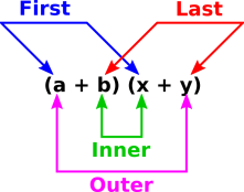 Figure 23
: FOIL = First + Outer + Inner + Last
8 Square Roots
8.1 Newton’s Method
If you can do long division, you can do square roots.
Most square roots are irrational, so they cannot be represented
exactly in the decimal system. (Decimal numerals are, after all,
rational numbers.) So the name of the game is to find a decimal
representation that is a sufficiently-accurate approximation.
We start with the following idea: For any nonzero x we know that
x÷√x is equal to √x. Furthermore, if s1 is
greater than √x it means x/s1 is less than √x. If
we take the average of these two things, s1 and x/s1, the
average is very much closer to √x. So we set
and then iterate. The method is very powerful; the number of digits
of precision doubles each time. It suffices to use a rough estimate
for the starting point, s1. In particular, if you are seeking the
square root of an 8-digit number, choose some 4-digit number as the
s1-value.
This is a special case of a more general technique called
Newton’s method, but if that doesn’t mean anything to you, don’t
worry about it.
8.2 First-Order Expansion
Note that the square of 1.01 is very nearly 1.02. Similarly, the
square of 1.02 is very nearly 1.04. Turning this around, we find the
general rule that if x gets bigger by two percent, then √x
gets bigger by one percent ... to a good approximation.
We can illustrate this idea by finding the square root of 50. Since
50 is 2% bigger than 49, the square root of 50 is 1% bigger than 7
... namely 7.07. This is a reasonably good result, accurate to better
than 0.02%.
If we double this result, we get 14.14, which is the square root of
200. That is hardly surprising, since we remember that the square
root of 2 is 1.414, accurate to within roundoff error.
9 Simple Trig Functions
Sine and cosine are transcendental functions. Evaluating them will
never be super-easy, but it can be done, with reasonably decent
accuracy, with relatively little effort, without a calculator.
In particular:
- You can always start with a zeroth-order approximation: For
angles near zero, the sine will be near zero. For angles near
90∘, the sine will be near 1. For angles near 30∘, the sine
will be near 0.5, et cetera.
- You can draw a graph, using the anchor points in equation 8 as a guide. You can then use graphical interpolation to
obtain values for any angle.
- A simple Taylor series gives a result accurate to 2.1% or
better using only a couple of multiplications. Remember to express
the angle in radians before using these formulas.
The following facts serve to “anchor” our knowledge of the sine
and cosine:
|
| |
| |
sin(0∘) | | = | | | | = | | 0 | | = | | cos(90∘) | | |
(8a)
|
|
| |
sin(30∘) | | = | | | | = | | 0.5 | | = | | cos(60∘) | | |
(8b)
|
|
| |
sin(45∘) | | = | | | | = | | 0.70711 | | = | | cos(45∘) | | |
(8c)
|
|
| |
sin(60∘) | | = | | | | = | | 0.86603 | | = | | cos(30∘) | | |
(8d)
|
|
| |
sin(90∘) | | = | | | | = | | 1 | | = | | cos(0∘) | | |
(8e)
|
| | |
|
Actually, that hardly counts as “remembering” because if you ever
forget any part of equation 8 you should be able to
regenerate it from scratch. The 0∘ and 90∘ values are
trivial. The 30∘ is a simple geometric construction. Then the
60∘ and 45∘ values are obtained via the Pythagorean theorem.
The value for 45∘ should be particularly easy to remember,
since √2 = 1.414 and √½ = ½√2.
The rest of this section is devoted to the Taylor series. A low-order
expansion works well if the point of interest is not too far from the
nearest anchor.
- For angles between −10∘ and +10∘, the approximation
sin(x)≈x is accurate to better than 0.51%. This is a
one-term Taylor series. Let’s call it the Taylor[1] approximation.
It is super-easy to evaluate, since it involves no additions and no
multiplications, or at most one multiplication if we need to convert
to radians from degrees or some other unit of measure. See
equation 9c and the blue line near x=0 in figure 24.
- For angles from 25∘ to 65∘, all the points are with a
few degrees of one of the anchor points in equation 8.
This means the first-order Taylor series is accurate to better than 1
percent in this region. We can call this the Taylor[0,1]
approximation. It requires knowing the sine and the cosine at the
nearest anchor point ... which we do in fact know from equation 8. See equation 13 and the blue line in
figure 24.
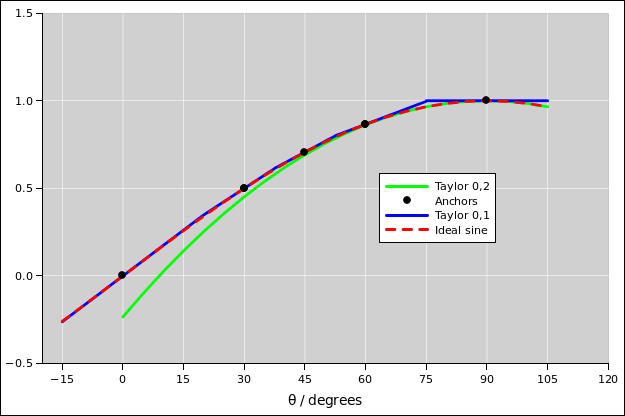 Figure 24
: Piecewise 1st-Order Taylor Approximation to Sine
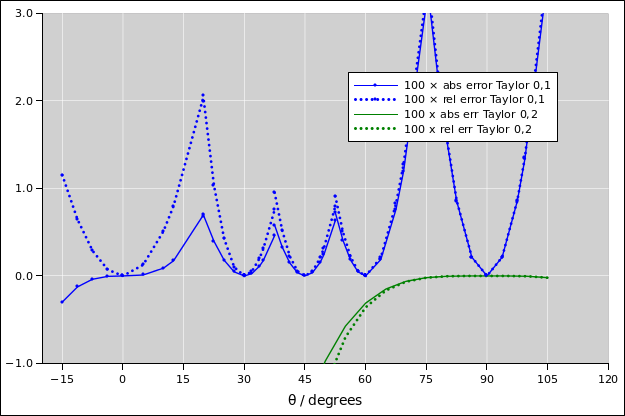
- For a rather broad range of angles near the top of the sine,
from 65∘ to 115∘, the approximation sin(x)≈1−x2/2
is accurate to better than half a percent. This is a second-order
Taylor series with only two terms, because the linear term is zero.
Let’s call this the Taylor[0,2] approximation. See equation 9e and the green line near x=90∘ in figure 24.
- This leaves us with a region from 10∘ to 25∘ that
requires some special attention. Options include the following:
For most purposes, the best option is to use the Taylor[1,3]
approximation anchored at zero. This requires a couple more
multiplications, but the result is accurate to better than 0.07%.
If you really want to minimize the number of multiplications, we can
start by noting that the Taylor[1] extrapolation coming up from zero
is better than the Taylor[0,1] extrapolation coming down from
30∘, so rather than using the closest anchor we use the 0∘
anchor all the way up to 20∘ and use the 30∘ anchor above
that. This has the advantage of minimizing the number of
multiplications. Disadvantages include having to remember an obscure
fact, namely the need to put the crossover at 20∘ rather than
halfway between the two anchors. The accuracy is better than 2.1%,
which is not great, but good enough for some applications. The error
is shown in figure 25.
There are many other options, but all the options I know of involve
either more work or less accuracy.
The spreadsheet that produces these figures is given by
reference 8.
Here are some additional facts that are needed in order to carry out
the calculations discussed here.
|
| |
1∘ | | = | | 17.4532925 milliradian | | | |
(9a)
|
|
| |
1 radian | | = | | 57.2957795∘ | | | |
(9b)
|
|
| |
sin(x) | | ≈ | | x | | for small x, measured in radians | |
(9c)
|
|
| |
cos(x) | | = | | sin(π/2 − x) | | for all x | |
(9d)
|
|
| |
| | ≈ | | 1 − x2/2 | | for small x, measured in radians | |
(9e)
|
|
Last but not least, we have the Pythagorean trig identity:
and the sum-of-angles formula:
|
sin(a + b) | | = | | sin(a)cos(b) + cos(a)sin(b) |
| (11)
|
If you can maintain even a vague memory of the form of equation 11, you can easily reconstruct the exact details. Use the
fact that it has to be symmetric under exchange of a and b (since
addition is commutative on the LHS). Also it has to behave correctly
when b=0 and when b=π/2.
If we assume b is small and use the small-angle approximations from
equation 9, then equation 11 reduces to the
second-order Taylor series approximation to sin(a+b).
|
sin(a + b) | | ≈ | | sin(a) + cos(a) b − sin(a) b2/2 | | for small b, measured in radians |
| (12)
|
If we drop the second-order term, we are left with the first-order
series, suitable for even smaller values of b:
|
sin(a + b) | | ≈ | | sin(a) + cos(a) b | | for smaller b, measured in radians |
| (13)
|
You can use the Taylor series to interpolate between the values given
in equation 8. Since every angle in the first quadrant
is at least somewhat near one of these values, you can find the sine
of any angle, to a good approximation, as shown in figure 24.
10 References
-
-
John Denker,
“Balancing Reaction Equations using Gaussian Elimination”
www.av8n.com/physics/gauss-elim.htm -
John Denker,
“Psychrometric Charts, and the Evil of Axes”
www.av8n.com/physics/axes.htm -
Douglas Isbell, Mary Hardin, Joan Underwood
“MARS CLIMATE ORBITER TEAM FINDS LIKELY CAUSE OF LOSS”
http://mars.jpl.nasa.gov/msp98/news/mco990930.html
-
Google Calculator. Example: furlongs per fortnight,
converted to SI units:
http://www.google.com/search?q=1+furlong+per+fortnight+in+m/s -
John Denker,
“Learning, Remembering, and Thinking”
www.av8n.com/physics/thinking.htm -
John Denker,
“Long Multiplication Videos”
www.av8n.com/physics/long-mult.htm -
John Denker,
“Long Division Video”
www.av8n.com/physics/long-div.htm -
John Denker,
“spreadsheet for checking trig approximations
./trig-approx.xls