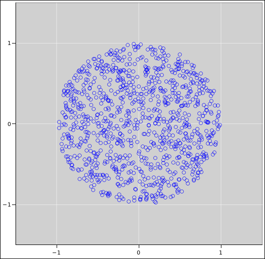
Figure 1: Uniform Distribution over the Unit Disk
We want the ability to generate some random numbers with a specified distribution. We shall see that there is a simple yet powerful and completely general way of doing this. Examples where this comes in handy include:
The solution presented here goes by various names including “inverse transform sampling” as discussed in reference 3 and references therein.
Suppose we want to construct some data, randomly distributed over the unit disk.
The derivation goes like this: The amount of probability within a circle of radius r goes like r2, as r goes from 0 to 1. That tells us the cumulative probability distribution, P(r) = r2.
For reasons that will be explained in section 2, we are interested in the functional inverse, namely r(P) = √P. We can implement the calculation as follows:
        r = sqrt(rand());
        theta = 2*pi*rand();
        x = r*cos(theta);
        y = r*sin(theta);
That’s all there is to it. The result is shown in figure 1.
As a prerequisite, we assume that you (i.e. your computer) can already generate random numbers with a uniform distribution on the interval (0,1). For details on how to generate such numbers with very high quality, see reference 4. For an introduction to the fundamental principles of probability, see reference 5.
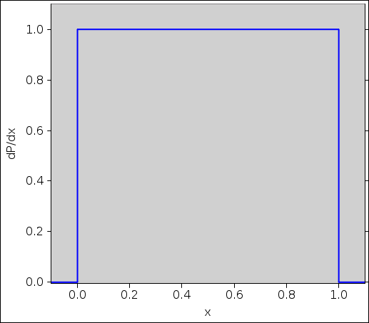
Figure 2 shows the probability density for a rectangular distribution.
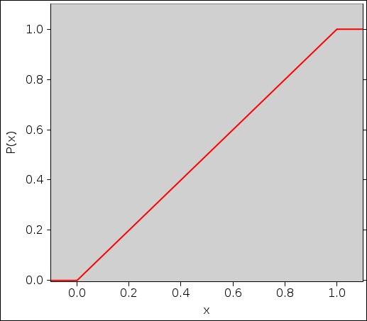
Similarly figure 3 shows the cumulative probability distribution function associated with a probability density that is rectangular, i.e. uniform over some interval.
Terminology note: We are using P(x) (with a capital P) to denote the cumulative probability distribution function. Specifically, P(x) is the total amount of probability measure to the left of x. The probability density is then dP/dx.
I am aware that many people think of the probability density (as shown in figure 2) as “the” probability, and denote it by P or p. However, there are a lot of probabilities in the world, and I am within my rights to use P to denote the cumulative probability distribution function, as shown in figure 3.
Strategy note: Whenever doing anything tricky (or even slightly tricky) with probabilities, it is good practice to think about the probability measure. This is the foundation, the mathematical bedrock, upon which our understanding of probability is based, as set forth in reference 6. A nice easy-to-understand yet sophisticated presentation can be found in reference 7. Probability is always the probability of some set. In the present example, the thing we have been calling P(x) is shorthand for P{r|r≤x}. If there is ever any doubt, we can rely on the set-theoretic formulation and be confident that we are saying something formal and precise.
Terminology note: In mathematics, the terms “distributed”, “distribution”, and “probability distribution” are used rather loosely, but the special two-word term “distribution function” is usually defined quite narrowly: It refers to the cumulative probability distribution function and nothing else, according to most authorities. This combination of looseness and strictness is quite inconsistent with the rules of ordinary English language. As an example, if you play by the math rules, the probability density function should never be called the “probability density distribution function”.
To be safe:
If you are speaking of the cumulative probability distribution function, put the word “cumulative” in there. According to the math rules, it’s redundant, but sometimes redundancy is better than ambiguity. If you are speaking of anything other than the cumulative probability distribution function, don’t say “distribution function”. If you use the word “distribution”, leave out the word “function” ... or vice versa.
Recall that our task for today is to transform one probability distribution into another. As a warm-up exercise, let’s practice transforming one uniform density x into another uniform density z. There are many ways of doing this.
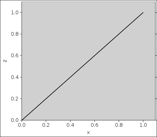
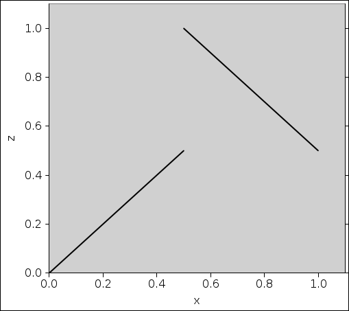
The simplest approach is the mapping shown in figure 4. That is, we just draw a random number x and use it to construct a numerically-equal random number z.
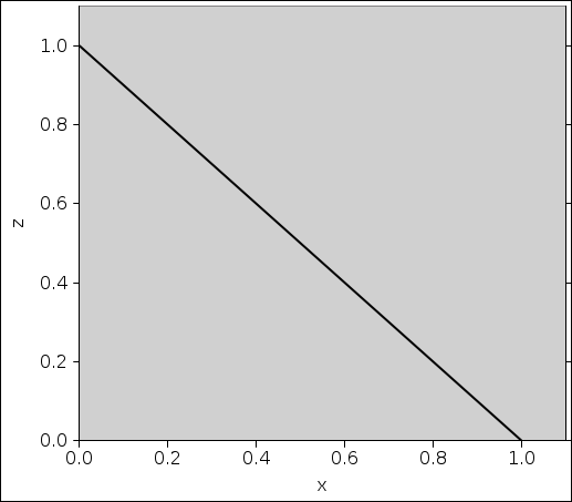
The mapping shown in figure 5 works just as well. We draw a random number x and use it to construct the random number z = 1.0−x.
We can combine the two previous approaches, as shown in figure 6. That is, if x is in the first half of the interval, we apply the mapping z=x, and in the second half of the interval, we apply the mapping z=1.5−x. Even though the mapping is discontinuous, it maps a uniform distribution dP/dx to a uniform distribution dP/dz. It maps the unit interval x ∈ [0,1] to the unit interval z ∈ [0,1].
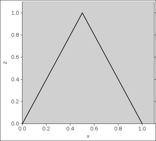
Things get even more interesting in figure 7. The first half of the x-interval gets spread over the entire z-interval. Note that the slope of the mapping function is larger than it was in the previous examples. This causes the probability to be spread thinly, and if this were the entire story, the z probability density would be only half of what it should be. However, we also map the second half of the x-interval onto the entire z interval, and if you add up both contributions, the z probability is just what it should be.
There are infinitely many additional ways of mapping one probability distribution to another.
However, we shall see that we can do everything we need to do using only monotone-increasing mappings, so figure 4 is our “preferred” mapping.
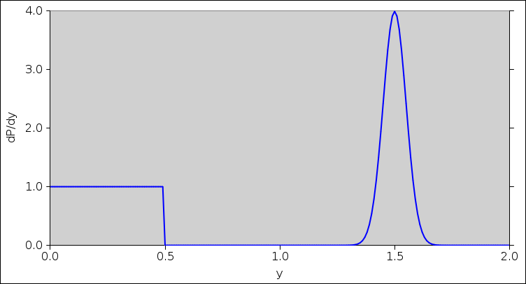
Again: our task for today is to transform one distribution to another. The interesting case involves transforming a uniform distribution into a non-uniform distribution. By way of example, let’s consider the probability density shown in figure 8.
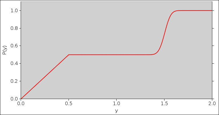
The corresponding cumulative probability distribution function is shown in figure 9.
Let’s be clear: We are given the distribution [either P(y) or dP/dy] as our assigned goal. We are also given a random number generator that will generate a uniform density dP/dx. Our task is to find a suitable mapping from x to y.
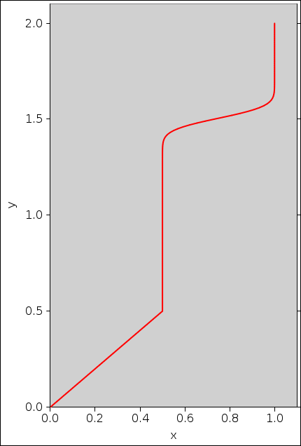
Without further ado, I will assert that the solution is shown in figure 10 ... and then we can discuss why this is correct.
The curve in figure 10 is just the functional inverse of P(y). If we were assigned P(y), all we need to do is invert it. Or, if we were assigned dP/dy, we integrate it to find P(y) and then invert.
To understand this result, it helps to have a clear understanding of what x means. Suppose we draw a random number x, and we get the value x=0.65; what does that value mean? Clearly this x-value has nothing to do with the probability density, because the density is uniform, and all x-values would have the same meaning, regardless of value. However, we can say something intelligent in terms of the cumulative distribution function. When x=0.65, it means that 65% of the probability measure lies to the left of x.
Now the trick is, we have constructed things so that when 65% of the x-measure lies between 0 and x, 65% of the y-measure lies between 0 and y. What could be simpler than that? This is based on y(x) as given by figure 10.
To say the same thing in other words:
| when | x | goes from | 0 | to | 1 |
| P(x) | goes from | 0 | to | 1 | |
| P(y) | goes from | 0 | to | 1 | |
| y | goes from | ymin | to | ymax |
To say the same thing yet again, we draw a value for x. This x is related (identically) to P(x) which is related (identically) to P(y). Then all we need to do is invert P(y) to find y.
As we have just seen, the situation is most easily understood in terms of the cumulative probabilities P(x) and P(y), but if you want to understand it in terms of the densities dP/dx and dP/dy, we can do that too.
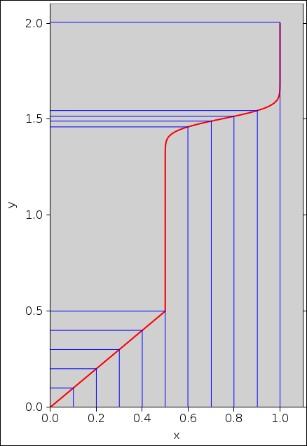
Figure 11 is the same as figure 10 except that some contour-lines have been added. The point is to emphasize the idea of measure. In particular, we require that all the x-measure be mapped to y-measure.
Note on interpreting this figure: The probability density is represented by the number of contours per unit length. For example, there is a large probability density near y=1.5 and a very small probability density near y=1.0.
Among other things, every contour line starts on the x-axis and ends on the y-axis. None of them get lost. Figuratively speaking, contour lines are conserved. Mathematically speaking, probability measure is conserved. Therefore this procedure upholds the normalization condition:
| ∫ |
| dy = | ∫ |
| dx (1) |
but there is much more going on than that. Equation 1 applies merely in an average or collective sense to all the probability. In contrast, we can make much stronger, much more detailed statements about the fate of individual parcels of probability measure:
If you are interested in the densities, it is the slope that matters in figure 11. For example, take a look at the middle portion of the curve, which has a near-infinite slope. Specifically, a small patch of probability-measure taken from the small interval x∈[0.5, 0.501] will get spread out over the huge interval y∈[0.5, 1.35]. This thinly-spread probability measure corresponds to a small probability density, as desired in this range of y, in accordance with figure 8.
We can formalize this mathematically, as follows. We see a mapping function y = f(x). Any such mapping will uphold the following rule:
| = ∑ | ⎪ ⎪ ⎪ ⎪ |
| ⎪ ⎪ ⎪ ⎪ |
| (2) |
where the sum runs over all (x,y) points such that y=f(x). Look at figure 7 to see why this summation is sometimes needed. On the other hand, since we are restricting our attention to monotone mapping functions, we can drop the sum and drop the absolute value bars from this expression. Then we can write:
| (3) |
where we have used the fact that dP/dx is uniform and normalized to unity.
Equation 3 re-expresses what we said earlier: if we are given the probability density dP/dy, we integrate it to find x(y). Then we invert that to find the desired mapping y(x).
The two main steps in the process are finding P(y) (by integrating dP/dy if necessary), and then finding the functional inverse.
There are various ways to do integrals:
I like doing them by computer. Macsyma is good at doing integrals. More to the point, an ancestral version of Macsyma, going by the name Maxima, is available for free. It is not as sophisticated as Macsyma, but it is plenty good enough for the sort of integrals I normally do. Example:
(%i1) foo: r*r*exp(-r);
                                    2   - r
(%o1)                              r  %e
(%i2) bar: integrate(foo,r);
                                2              - r
(%o2)                       (- r  - 2 r - 2) %e
(%i3) subst(r=0, bar);
(%o3)                                 - 2
(%i4) subst(r=9e99, bar);
(%o4)                                 0.0
(%i5) string(bar);
(%o5)                         (-r^2-2*r-2)*%e^-r
Installing Maxima is trivial on the usual Linux distributions. I’m told there is also a windows version. See reference 8. The manual is conveniently online; see reference 9.
For me, using the computer is much faster than doing integrals by hand. It is quicker even than looking things up in a book. It is also more reliable. If I correct a mistake or change my mind, I can make a small change in the script and re-run the whole thing at near-zero cost. Last but not least, using the string() function I can put the results into a format that can be cut-and-pasted into a c++ or java program with only minor transliteration.
Maxima will not always simplify things the way you want, but if you simplify them by hand, the computer will do an excellent job of verifying that your simplified version agrees with the original.
There are some functions where the inverse has a nice closed-form expression. For example, the inverse of exp() is ln(). More generally, the Weibull distribution has a closed-form inverse ... which is particularly nice because it includes several interesting distributions as special cases. See reference 10.
There are other functions where you can obtain a closed-form inverse by means of a trick. For example, the two-dimensional Gaussian is easier to deal with than the one-dimensional Gaussian. In the context of Gaussian-distributed random numbers, this is used in the clever Box-Muller transform; see reference 11.
There are many other functions where there is little hope of finding a closed-form expression for the inverse function. However, if you need the inverse function for use in a computer, there exist sure-fire methods for inverting any invertible function:
One way is to tabulate the function and then interpolate. If you can tabulate the function y(x), you can just as easily tabulate its inverse function x(y); all you need to do is swap the abscissa and ordinate when building the interpolation table. This is the general rule for inverting any tabulated function, provided it is one-to-one. Here’s a simple example:
| Function | Inverse Function | |||||||||||||||||||||||||||||||||||||
| y(x) | x(y) | |||||||||||||||||||||||||||||||||||||
|
| |||||||||||||||||||||||||||||||||||||
Another way to invert any invertible, computable function is by binary search.
These methods can be combined: You can use an interpolation table to get close, and then evaluate the obverse function to verify the accuracy of the interpolation process, and/or refine the result via binary search.
All these methods can be combined with plain old algebra. For example, in atomic physics, the radial part of the cumulative probability for a hydrogenic orbital can be expressed as
| P = 1 − f(r) exp(−2r/N) (4) |
where N is the principal quantum number (“shell number”), and where f(r) is a polynomial. We can rewrite this as
| (5) |
In this expression, given P we can calculate ln(1−P), so the only thing we need to tabulate is the polynomial. Actually we want the functional inverse of the polynomial, so we must tabulate f (or ln(f)) as a function of P, not as a function of r. This is easy to do.
The point here is that it is easier to accurately interpolate a polynomial (which is a relatively weak function of r) than an exponential (which is a much stronger function of r).
The general rule is to separate out the dominant contribution to the function of interest ... then tabulate and interpolate whatever is left.