1  Overview

Any system of N linear equations in N unknowns can be solved systematically and efficiently (assuming it was solvable to begin with). The classic method for doing this is Gaussian elimination, also known as the Gauss-Jordan algorithm. This general topic is known as linear algebra.

• For smallish N, the method is easy to carry out using only pencil and paper. (Remember that Gauss worked in the early 1800s, long before computers were available.)
• For any reasonable N, the method can also be carried out using a simple spreadsheet application, or various other computer programs, in less time that it takes to tell about it.
• Linear algebra can also be used to map out the solution space when there are N equations in more than N unknowns.
• This is useful for balancing chemical reaction equations. Reactions that are widely considered “difficult” or “impossible” to balance can be solved easily.

*   Contents

• 1  Overview
• 2  An Illustrative Example : Cadmium Oxidation
  • 2.1  Setting Up
  • 2.2  Gaussian Elimination using Pencil-and-Paper
    • 2.2.1  Uphill
    • 2.2.2  Downhill
  • 2.3  Spreadsheet Solution
• 3  Multi-Dimensional Solution Space
  • 3.1  Peroxide + Permanganate
  • 3.2  Positive Solutions
• 4  Discussion
  • 4.1  The Normal Case
  • 4.2  Unbalanceable
  • 4.3  Overdetermined
  • 4.4  Underdetermined
  • 4.5  The Pseudo-Inverse Method
  • 4.6  Products Masquerading as Reactants; Negative Coefficients
• 5  Why and How to Be Careful
• 6  References

2  An Illustrative Example : Cadmium Oxidation

2.1  Setting Up

We shall see that even a somewhat complicated-looking reaction can be balanced easily. I will do an example, and explain the rules as I go along. The following reaction¹ – taken from reference 1 – will serve as good illustration:

The first rule is to write the reaction using undetermined coefficients, as was done in equation 1, where the coefficients are a, b, c, x, y, and z. This is in preference to writing just the “skeleton” of the reaction, in which the coefficients are omitted entirely, as in equation 2.

The skeleton may have the superficial attraction of brevity, and you need to recognize skeletons because they commonly appear in books and elsewhere, but for present purposes we really need to see the coefficients. In particular, equation 2 does not assert that the coefficient in front of each reactant is unity; it doesn’t say anything about the coefficients. We need the coefficients, as in equation 1, because we want to write equations involving them:

So, we have 5 equations in 6 unknowns. This is as it should be. It is of the form N linearly independent equations in N+m unknowns, where in this case N=5 and m=1. The fact that the number of degrees of freedom (m) is greater than zero means the solution will not be unique. There will be an m-dimensional set of solutions. In our case, the solution-set will contain all possible ways of scaling-up or scaling-down the recipe. (If you want to write the solution in standard form, that’s allowed, but we should not pretend that’s the only solution.)

Equation 3 writes the equations in old-fashioned mathematical format. Each variable a, b, c, et cetera is written in its own column. After a while, you realize you can save time by just writing the numerical factors in each column, without bothering to write the name of the variable, so long as you are careful to write each number in the proper column. Here’s what that looks like:

The correctness of equation 4 is most easily verified by looking at each column. For example, we know b is the coefficient in front of HNO₃, so it is good to see 1,1,3 in the H, N, and O rows of the appropriate column.

With a little practice, you will be able to write equation 4 just by looking at the original reaction equation, without bothering with equation 3.

If you are working the problem using pencil and paper (as opposed to a computer), it is recommended that you pounce on any coefficients that have obvious solutions. Looking at equation 3 or equation 4, it is pretty obvious that a = x. Similarly, it is pretty obvious that y = 2x, since the LHS is manifestly charge-neutral, no matter what the values of the coefficients, and the NO₃^– ion is the only thing on the RHS that could possibly balance the charge of the Cd⁺⁺ ion.

That means we can write down the partial solution

and proceed to solve for the remaining variables. That leaves us with:

We have gotten rid of the a and x columns, since we know those based on equation 5. We have gotten rid of the Cd and charge rows, because we have already used those in finding the partial solution, so they don’t tell us anything we don’t already know. Once again we have a system of N equations in N+m unknowns, where N is now reduced to 3, and m is still 1.

The next step is to shuffle things around so that there are N columns on the LHS and m columns on the RHS. Let’s flip the z variable to the other side of the “=” sign. That gives us:

The subscript on z_r is to remind us that it represents the amount of NO on the RHS of the reaction equation, even though we are writing it on the LHS of equation 7.

Unless there is something seriously wrong with the original reaction equation, it doesn’t much matter which m columns you choose for the RHS.

The only thing that is even halfway tricky about this is that you must change the sign on each number when it gets flipped from one side of the equation to the other. Remember, what we are doing is not magic. It is well-founded in the axioms of arithmetic. In this case we are subtracting the same thing from both sides of the equation.

2.2  Gaussian Elimination using Pencil-and-Paper

2.2.1  Uphill

The next phase can be considered the “uphill” phase of the Gaussian elimination algorithm. The goal of this phase is to convert the matrix in equation 7 to upper-triangular form. We do this by subtracting one row from another, step by step, as many times as necessary, so as to create strategically-placed zeroes in the result.

The basic motto for this phase is “multiply by ... and add”. (We will formulate an improved motto in a moment.) The basic idea is to take one row, multiply it by some constant, and add it to another row. We choose the constant so as to create a zero in a useful place.

As a first application of this motto, we multiply the first row by -1 and add that to the second row. That gives us:

The purpose of this step is to create a zero in the leftmost column of the bottom row.

You will notice that I have grayed-out one row of the table. If you were doing this with pencil and paper, you would just lightly cross out that row. We won’t be needing that row again, but as a general principle that you should never erase any of your work ... I recommend keeping it around, to facilitate checking your work.

Also over on the right, in square brackets, I have written a hint as to where the new line came from: The first number (2 in this case) indicates that this is a replacement for line #2, and the other number (1 in this case) indicates that line #1 was also involved in the construction of this line. This is not necessary, just recommended, to facilitate checking your work.

The rule here is that we have combined two lines to create a new one, and the new line should be considered a replacement for one of the old lines. It doesn’t really matter which of the old lines you cross out. Just pick one. The method will work either way.²

Continuing along this road, we multiply the first line by -3 and add it to the third line. That gives us:

The purpose of this step was to create another row with a zero in the leftmost column. Before we had only one non-gray row with a zero in the leftmost column, and now we have two. This is good. This is progress.

The bottom two rows in equation 9 can be viewed as two linear equations in two unknowns, and can be solved by continuing the tried-and-true Gaussian elimination process. We are still in the uphill phase of the process.

The second-best way to proceed would be to multiply the next-to-last row by −5/2 and add that to the last row. But paper is cheap, multiplication is easier than division, and integers are nicer than fractions, so many people find it advantageous to separate this step into two half-steps. We cross-multiply. Rather than multiplying the last line by 2/(−5), we multiply the last line by 2 and multiply the other line by −5.

The first half-step is to multiply the last line by 2, which gives us:

To finish the step, we multiply line #4 by -5 and add it to line #6. That gives us:

The refined motto is: “Cross-multiply and add”. If you want to minimize the number of multiplications, you should not cross multiply, but rather should multiply by a ratio. On the other hand, if you want an integer result, cross-multiplication is the correct move.

2.2.2  Downhill

At this point we have reached an important milestone. We have succeeded in putting the matrix into upper-triangular form. (As always, we are ignoring the crossed-out rows.) We now begin the downhill phase of the calculation.

The purpose of this phase is to convert the matrix into fully diagonal form. The motto for the downhill phase of the calculation is “Use a singleton row to clean out its column.” That is, find a row where the nonzero element is in the Mth column, and use that to zero out the Mth column of all other rows.

The multiply-and-add operation is easy for two reasons: Firstly, multiplication by zero is easy. Secondly, addition of zero is easy, and means there will be no side-effects on columns other than the one you are working on.

The first step of the downhill phase is to read out the result from the bottom row, which tells us directly that 3z = y, hence z = y/3.

The next step is to multiply line #4 by 3. That gives us:

In equation 12, the “triangular” structure is not quite so obvious, but the same strategy applies: Use the short row first, because the multiplication and addition are particularly easy, and have no side-effects on other columns. The next step is to add line #7 to line #8:

We now have two singleton rows. Each full step in the downhill phase is guaranteed to produce a new singleton row. Each singleton row can be used to clean out a column.

At this point the remaining equations are so simple that you could solve them in your head, but it’s just as each to keep going with the algorithm. The final step uses line #9 to clean out the c column of the top row in equation 13. So the final form of the tableau is:

so you can see we have succeeded in putting the matrix into diagonal form. This completes the Gaussian elimination. You can pick off the values of all the coefficients from equation 14. Every coefficient is known in terms of some multiple of y. (The coefficient y is special because it is the one we chose to put on the RHS of equation 7.)

We can obtain a preliminary solution by arbitrarily picking a value for y. We could pick y=1 or any other value; changing the value corresponds to “scaling the recipe”. We can save ourselves a step if we choose y equal to the LCM (least common multiple) of the numbers on the diagonal in equation 14. The resulting solution is correct but we call it preliminary because it might not be in standard form.

Let’s collect results:

The fact that c is negative tells us that we guessed wrong when we wrote the H₂O term on the LHS of the reaction; we need to move it to the RHS, for reasons discussed in section 4.6. This will flip the sign of the coefficient.

You can see why we chose the LCM as the y-value. The numbers from the diagonal appear in the denominators in the second column of equation 15, while y appears in the numerator. This guarantees that the coefficients in the third column are integers.

To obtain a solution in lowest terms, calculate the GCD (greatest common divisor) of the coefficients, then divide through. In our case the GCD is already 1, so this step doesn’t change anything.

For our example, we obtain:

This equation is even easier to verify than it was to derive. Please take a moment to convince yourself that this result is balanced w.r.t cadmium, hydrogen, nitrogen, oxygen, and charge. You can do this in your head; it requires little more than counting.

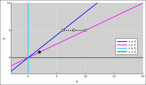
The entire solution set for the b and y coefficients is shown in figure 1. For any value of y, there is a definite value of b required to balance the equation, as shown by the magenta line. The solution set starts at (0,0) and extends without limit in the upper-right direction. The solution in standard form is shown by the black circle at the point (y,b) = (6,8).

Figure 1: Cd Solution Set

2.3  Spreadsheet Solution

When N is larger than 4 or 5, it might be quicker to solve the equations using a computer. You don’t need to know about Gaussian elimination to do this; you just use the matrix-inverse function (which uses Gaussian elimination internally). This function is available in garden-variety spreadsheet programs and elsewhere. There are also more-specialized programs specifically targeted at chemistry applications.

A working example of a reaction-balancing spreadsheet can be found in reference 2. You can modify that one, or construct your own as follows: Type the coefficients from equation 7 into the spreadsheet, into a N×(N+1) block of cells, such as D8:G10. Now highlight (i.e. select) another N×(N+1) block of cells, perhaps D13:G15. Type in the formula =mmult(minverse(D8:F10),D8:G10) and hit Control-Shift-Enter. (Note that plain old “Enter” will not suffice.) That’s the only halfway tricky step.

Note that the argument to minverse is the N×N array that comes from the LHS of equation 7, while the second argument to mmult is the full N×(N+1) array, including both sides of equation 7.

The result will be a N×N unit matrix alongside a 1×N vector of coefficients, which are the answers. (The unit matrix doesn’t tell you anything very interesting, but it is super-easy to compute, and serves as useful confirmation that the method is working.) You may need to multiply the vector of coefficients by something in order to bring them into standard form.

Let’s do the problem again, using the reaction equation directly, with no clever simplifications. Here is the equation again, copied from equation 1:

The coefficients are:

Remember the rule: any coefficient that starts out on one side of the “→” sign in equation 17 and gets shuffled over to the other side gets its sign flipped (such as x, y, z, and a in equation 18).

The solution looks like this:

The advantage of doing it this way is that the coefficients that get typed into the computer correspond directly to the original reaction equation, which makes it easy to check that they are correct. Any clever simplifications that you apply make the checking more difficult. There is no disadvantage to his approach, because computer can do a N×N system of linear equations in practically zero time, even for rather large N. (Doing it by hand for large N would not be so much fun.)

To put the results into standard form, proceed as follows: Choose a raw upscaling factor. The exact value doesn’t matter, so long as it contains enough factors, and isn’t so huge as to be not representable as an exact integer. If you can’t think of anything cleverer, use 10 factorial, because that contains several different prime factors. Put it in a cell somewhere. Then in a new column somewhere, multiply the preliminary results from the matrix calculation by the raw upscale factor, and use the abs(round(..., 3)) function to round off the product. Then use the gcd(...) function to find the greatest common divisor of all the rounded products. The cooked scale factor is the raw factor divided by the gcd. In another column somewhere, multiply the preliminary results by the cooked factor. This should give the integerized results in lowest terms. If the results are still not integers, multiply the raw factor by something that will make them integers.

The rounding step is necessary, because the matrix calculation commonly produces numbers of the form 1.9999999999999, which the spreadsheet will display as 2, but which the gcd(...) function will not recognize as integers. (There exist integer-only versions of the Gaussian elimination algorithm, based on cross-multiplication, but ordinary spreadsheets applications don’t know about them.)

In some spreadsheet versions, the abs(...) function is needed because the gcd(...) function fails on negative numbers. There is no excuse for this failure, but be have to work around it.

3  Multi-Dimensional Solution Space

3.1  Peroxide + Permanganate

The following reaction is used in the real world to titrate the amount of hydrogen peroxide.

Tangential remark: One remarkable point is that even though hydrogen peroxide is normally considered an oxidizing agent (and therefore gets reduced), in this case it is interacting with a more powerful oxidizing agent, and in fact the permanganate gets reduced. However, for present purposes, we don’t need to worry about this.

This reaction is particularly interesting because it has multiple degrees of freedom.

The problem is, equation 19 is not sufficient to specify what goes on during the titration experiment. There are a lot of things that could happen, and without further information we have no way of knowing which of these things actually happens.

The task of balancing equation 19 is ill-posed. The symptom is that when we try to balance it, we get 4 equations in 6 unknowns ... which immediately raises red flags. The four equations represent conservation of hydrogen, oxygen, manganese, and charge. There are six parameters, namely a, b, c, x, y, and z.

This leaves us with two degrees of freedom. The solution-set will be a two-dimensional space. Even if we freeze one of the coefficients, to remove the overall scale freedom, we are left with one degree of freedom, and infinitely many solutions.

Here is one of the solutions, as you can easily verify:

where we have written the numerical value for each parameter underneath the parameter. This is nonstandard, but easier to read, once you get used to it.

For reasons that will become clear in a moment, in connection with equation 23, we will find it convenient to scale up this reaction by a factor of five, so we rewrite it as:

The reaction in equation 20 is entirely legitimate. It represents the decomposition of hydrogen peroxide. There are lots of ways this reaction can proceed as written. When catalyzed, it is vigorously spontaneous.

This equation is well balanced. Presumably this reaction does not proceed as written. I suspect it is energetically disfavored, or some such. However, if your only task is to balance the equation, this is a solution.

More generally, any convex combination of equation 20 and equation 22 is a way of balancing equation 19. To say the same thing another way, equation 20 and equation 22 are basis vectors that span the solution space.

For the titration application, the desired reaction is the following:

which can be thought of as a 50/50 combination of equation 21 plus equation 22.

It must be emphasized that the task of balancing equation 19 remains ill-posed. No sound method of “equation balancing” could possibly yield equation 23 as the solution, because no matter what you think the solution is, you can pick any real number (within limits) and add that much of equation 20 and get another solution. There are uncountably many ways of balancing the original equation, most of which have no particular stoichiometry.

To say the same thing another way: If you think you have a “method” that produces equation 20 directly from equation 19, you’re fooling yourself. Any alleged “method” that does not produce equation 20 as part of the solution-set is so sketchy that it doesn’t deserve the name “method”.

It is possible to engineer conditions so that the reaction described by equation 23 is favored and equation 20 is negligible in comparison. However, those conditions are not described by the original statement of the problem, equation 19. Equations are famously unable to read your mind. If you have in mind particular conditions, pathways, and rates, you need to write down equations that express what you are thinking ... before you start trying to balance the equations.

The actual mechanism that leads to the stoichiometry indicated in equation 23 is quite complex; see reference 3.

There are simple ways of solving underspecified problems using linear algebra. It can be done using pencil and paper, although a spreadsheet program speeds things up and may be more reliable. An example of this, applied to the peroxide-permanganate task, is included in reference 2.

The general idea is this: Given a system with N equations and N+m unknowns, write it as an N×(N+m) matrix. Then make a copy of the matrix, with the following modification: Arbitrarily pick m of the variables, move them to the RHS of the equation, and freeze them. Pick plausible values for them. Re-arrange the corresponding m columns of the matrix so that they appear on the right ... and multiply each of these columns by the corresponding frozen variable.

• Don’t forget this multiplication.
• The other N columns do not undergo any corresponding multiplication.

Any other columns on the RHS get moved to the LHS, and their matrix elements get their sign flipped in the process. The LHS is now an N×N matrix that can be inverted in the usual way.

Apply the inverse matrix to the entire N×(N+m) system. In the product, the m “extra” columns are vectors that span the solution-space.

In figure 2, the solution set for the x and y coefficients is the entire triangular-shaped wedge above the magenta line and below the blue line.

Figure 2: Peroxide+Permanganate Solution Set

If we freeze out the overall scale freedom by choosing y=5, there are still uncountably many ways of balancing the reaction, as shown by the dotted black line. The three circles on this line correspond to equation 21, equation 23, and equation 22.

The solid black dot corresponds to equation 20.

By way of contrast, you can see that ordinary, easy reaction equations (such as the cadmium oxidation reaction discussed in section 2) correspond to m=1, where the only degree of freedom is the overall scale. The only “corner” is the obvious endpoint, at the point where all the coefficients are zero, as we see in figure 1.

3.2  Positive Solutions

So far we have mostly emphasized the linear algebra involved in solving N equations in N+m unknowns. That’s fine, but the real problem we are trying to solve involves more than that. It also involves N+m inequalities, namely the requirement that each of the coefficients take on a positive value.

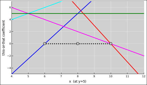
When there are more than one degree of freedom, i.e. when m>1, these inequalities impose some nontrivial structure on the solution set. This is why the solution set in figure 2 is a triangle and not the entire (x,y) plane. We have two degrees of freedom, so we get to choose x and y ... but there are some constraints on our choice. That is, after we choose x, we get to choose y independently of x if it is within the solution set but not otherwise.

We can understand this structure with the help of figure 3. The colored lines depict all six coefficients (including x) as a function of x, in the case where y is fixed at y=5. (There are only five lines visible, because two of the coefficients are numerically equal.) This corresponds to a cross-section through figure 2, taken along the contour of constant y=5. The dotted line in the two figures is the same, and indicates the set of all feasible solutions when y=5.

Figure 3: Peroxide+Permanganate Inequalities

In figure 3, we can see that the solution set is limited by the requirement that all of the coefficients must be positive.

This is useful, because it tells us how to find the corner cases when m=2. There are six tasks, each of which consists of solving one linear equation in one unknown, which is not much of a challenge. That is, we need to find the zero-crossing for each of the lines shown in figure 3. The largest upward zero-crossing and the smallest downward zero-crossing are the limits of the feasible region.

The curves in this figure were computed with the aid of the “basis x” and “basis y” vectors produced by doing the linear algebra, as shown on the spreadsheet. Note that if we were not worried about constraining the coefficients to be positive, we could have just added the x and y columns together, so that we had only one column on the RHS of the equation. The system is linear, so this would have given us perfectly good values for the coefficients corresponding to any chosen (x,y) point. It would, however, have complicated the task of finding the corner cases. That is, it would have complicated the constraint-satisfaction part of the task.

The corner cases are significant because they help us map out the boundaries of the solution set. Also note that we can use the set of corner cases as a new set of basis vectors. Any other solution can be written as a linear combination of the corner cases, using only non-negative coefficients, as we see in equation 20 and equation 22.

If m is greater than 2, you have to work a little harder to find all the corner cases. This is beyond the scope of this document. At some point it becomes a linear programming task.

4  Discussion

4.1  The Normal Case

Gaussian elimination follows a simple pattern: Basically you work your way down, cleaning out the columns one by one until the matrix is in upper-triangular form. Then you work your way back up, putting the matrix into diagonal form. With a little practice, you can do it very quickly with very high confidence in the results.

The work required goes roughly like N cubed, so a N=4 system is about twice as laborious as a N=3 system, and a N=5 system is about twice as laborious as a N=4 system.

There is nothing mysterious about Gaussian elimination. The validity of every step is based on the most basic laws of algebra: multiplying both sides of an equation by a constant, adding one equation to another, and things like that.

The most obvious advantage of this method is that it gives you a compact and tidy way of doing the algebra, and it gives you some guidance as to which equation should be multiplied by a constant, and which equation should be added to which other.

Each row of in the Gaussian elimination tableau is an equation with N+m variables ... we have just omitted the names of the variables for convenience.

4.2  Unbalanceable

Chemical reaction equations are supposed to have at least one degree of freedom, namely scale freedom.

If you ever encounter a system of N linearly-independent equations in N unknowns, there is something wrong. Mathematics tells us there are no degrees of freedom. Examples include equation 24 and equation 29. Unbalanceable systems are very bad news. They express a built-in contradiction. Such a system has no nontrivial solutions.

This typically results from an erroneous reaction equation. A common error is to write a reaction equation that fails to mention one of the reactants or one of the products. (This is particularly easy to do if H₂O is participating in the reaction.)

Here is an example:

There are three equations in three unknowns. Therefore we are expecting a single pointlike solution, not a family of solutions. The equations are:

If we scale things so that a=1, the first two equations tell us that x=1/3 and y=2, but the third equation is a contradiction because 6 is not equal to 4/3 + 2.

The only solution to equation 25 is the trivial solution, where (a,x,y) = (0,0,0).

To get out of this mess, you must find the correct reaction equation. Doing this requires knowing some actual chemistry, not just mathematics. As such, it is beyond the scope of this document ... but we can offer some illustrations of what might result from a proper analysis. Here is a first guess at a more-plausible replacement for equation 24:

This is at least balanceable:

which has the solution (x, y, z) = (1/3, 2, 4/3).

Depending on reaction conditions, it may well be that NO₂ would be evolved instead of O₂:

which is also balanceable.

The same logic applies to other examples, including the following:

Just as in equation 24, this is overdetermined. It cannot proceed as written. It would evolve excess oxygen in some form, which the RHS of the reaction equation fails to take into account.

4.3  Overdetermined

Taking things even further in the wrong direction, a system of more than N linearly-independent equations in N unknowns is said to be overdetermine. An overdetermined system has no solutions, not even the trivial all-zeros solution.

If you try to solve a system using Gaussian elimination, the process will fail. You will observe the following symptom: At some point when you attempt to clear out one of the entries, you will get a self-contradictory expression of the form 0 = k, for some nonzero k. This is an example of an ill-posed problem, as discussed in reference 4.

4.4  Underdetermined

All normal, practical chemical reaction equations have at least one degree of freedom, namely the obvious scale freedom. You can always scale-up or scale-down the recipe. Technically, that makes them mathematically underdetermined. That is to say, there are multiple ways of balancing the equation. This is not a problem. Scaling is real.

You can remove scale freedom by choosing to write the equation in “standard form”, but that is artificial. The chemicals don’t care whether or not you carry out the reaction using exactly one mole of this and two moles of that.

Sometime the system has multiple degrees of freedom – that is, scale freedom plus one or more additional freedoms.

• A classic, important system with multiple degrees of freedom is the following:

  a C + b  O2 →  x CO + y CO2              (30)

  where we have N equations in N+m unknowns; specifically, N=2 equations in N+m=4 unknowns, leaving us m=2 degrees of freedom. Even if you get rid of scale freedom, there is still another degree of freedom.

• Another interesting case where m=2 is the peroxide + permanganate titration discussed in section 3.1.
• Sometimes you encounter a less-obvious situation in which you nominally have E equations but alas not all of the equations are linearly independent. What really matters is not E (the number of equations) but N (the number of linearly independent equations). For example:

  a Fe+++ + b SCN− → c FeSCN++         1   0 = 1 [Fe balance]    0   1 = 1 [S balance]    0   1 = 1 [C balance]    0   1 = 1 [N balance]    3   −1 = 2 [charge balance]

  (31)

  That looks like E=5 equations in three unknowns, but really it is only N=2 linearly independent equations, because the C and N equations are identical to the S equation, and the charge equation is linearly dependent on the Fe and S equations.

  Practically speaking, Gaussian elimination is often the most efficient way to discover if a given system of equations contains hidden linear dependencies. If during one of the multiply-and-add steps, if the result is a row containing all zeros, there was a linear dependence in your initial set of equations.

• Sometimes equations are written in a way that is not scale-invariant. For example,

  a C + b  O2 →  x CO + (1−x) CO2              (32)

  leads to the equations

  a    b    =    1    x    [from]       1    0    =    1    0    [C]     0    2    =    2    −1    [O]

  (33)

  No matter what the value of x, we must have a=1. The recipe cannot be scaled up or scaled down. The explicit constant “1” on the RHS messes things up.

Whether you can succeed in solving an underdetermined system depends on how you define success. If you insist on finding “the” unique solution, that’s impossible. Since there is a family of solutions, the professional approach is to find a description of the entire solution-set.

You can always hide the scale invariance by arbitrarily setting m of the coefficients to some arbitrary value.

Also note that a system that is naturally nonsingular can become seemingly singular if you inadvertently cross out the wrong row during the Gaussian elimination procedure.

4.5  The Pseudo-Inverse Method

An elegant method for handling the general case, including ill-posed tasks, can be found in reference 5. An example implementing this method is included in reference 2.

There are several things to note:

• You can almost always get Gaussian elimination to work, and when it works, it is requires less effort than the pseudo-inverse method. However, sometimes when the task is ill-posed in a non-obvious way, you might need to do several Gaussian eliminations to figure out what the problem is. In such a case, it might be easier to use the pseudo-inverse method.
• The “g-inverse” mentioned in reference 5 is also known as a generalized inverse or pseudo-inverse. It is not necessarily unique. If you want uniqueness, the Moore-Penrose pseudo-inverse is a particular type of pseudo-inverse, which is unique.
• It is not always easy to calculate the pseudo-inverse. The “limit” method is well defined in theory but is often numerically unstable in practice. I calculate the pseudo-inverse two ways – denominator on the left and denominator on the right – because it is not a priori obvious which way is going to work better. Fiddling with the “epsilon” in the limit provides a useful check.
• The spreadsheet formula to calculate the pseudo-inverse is so complicated that I wrote a formula to calculate the formula.
• Reference 5 contains an amusing chronological list of 125 references, some dating back more than 100 years, on the topic of how to balance chemical reactions.
• The paper defines “the” problem to include the second part of the problem, namely finding the solutions with all non-negative coefficients, and claims to have solved “the” problem ... but does not actually address the second part. The linear algebra in the paper will blissfully give you negative coefficients as well as positive coefficients. Finding the non-negative solutions is not entirely trivial, especially when the solution-set has many degrees of freedom.

  In some cases it is important to uphold the reaction equation as written, and exclude negative coefficients. In other cases, it may be desirable to find all solutions, and then re-interpret negative coefficients as representing a different reaction, as discussed in section 4.6.

4.6  Products Masquerading as Reactants; Negative Coefficients

Consider again reaction equation 1, which we reproduce here:

The mathematical analysis produces a negative value for the coefficient d. That tells us the H₂O is really a product not a reactant, so we should rewrite the equation as

whereupon we obtain a positive value for the new parameter w.

Superficially, there is a simple rule: If you see a negative coefficient in front of an alleged reactant, it is really a product. You should move it to the other side of the reaction equation (which changes the sign of the coefficient). Similarly, if you see a negative coefficient in front of an alleged product, it is really a reactant. Move it to the other side.

At a deeper level, however, if you see a negative coefficient it should put you on guard. It indicates there was a misconception in the original reaction equation. Perhaps it was just a benign, isolated misconception, but perhaps not; perhaps it is only the tip of the iceberg. You should careful re-examine the situation, and do whatever you have to do to obtain the correct reaction equation.

Important remark: Stoichiometry and equation-balancing are simple mathematical exercises if – and only if – you can rely on the correctness of the reaction equation you are asked to balance. To say the same thing the other way: mathematics is not a viable substitute for understanding what chemistry is actually occurring.

5  Why and How to Be Careful

Gaussian elimination requires a lot of steps. Each step is extremely simple – a ten-year-old could do each step – but there are a lot of steps.

Suppose there are 11 rows in your tableau, as there are in equation 14. Each row requires a few very simple one-digit multiplications and one-digit additions. So all in all, there could be something like 100 elementary operations.

Now, suppose you can do each elementary operation with 95% reliability. Do you think this should be considered “grade-A” work, because 95% of it is correct? There’s a problem with that. At this rate, the probability that you will generate a fully-correct tableau is 0.95 to the 100th power, which is less than one percent!

You will know that you’ve made a mistake, because the coefficients you have calculated do not in fact balance the equation. This is your cue to re-do the problem, more carefully.

To turn the previous probability calculation on its head, if you want to be able to finish the tableau and have a 95% chance that the whole thing is correct, you need to perform each elementary operation with reliability 99.95%. That sounds like a pretty high probability, but there’s no reason why you can’t achieve it. Remember, each of the elementary operations is very simple.

So the question is: can you do simple things reliably?

Some standard advice to increase the convenience and/or reliability of your calculations can be found in reference 6.

Also note that if you do the problem once using the pencil-and-paper method and again using a computer, it increases your chance of catching a mistake. Certainly it is possible to make a mistake using either method, but with any luck you will make different mistakes, and thereby discover that something is wrong.

6  References

1.

John Denker, "Balancing Reactions w.r.t Charge and Atoms" ./balance-charge-atom.htm

2.

John Denker,
“Spreadsheet for Balancing Chemical Reactions”
./chem-balancing.xls

3.

Reuben H. Simoyi, Patrick De Kepper, Irving R. Epstein, and Kenneth Kustin,
“Reaction between permanganate ion and hydrogen peroxide:
kinetics and mechanism of the initial phase of the reaction”
Inorg. Chem. 25 (4), pp 538–542 (February 1986).

4.

John Denker "Ill-Posed Problems" ./ill-posed.htm

5.

“Ice B. Risteski”, “A New Approach to Balancing Chemical Equations”
SIAM Problems and Solutions (2007)
http://www.siam.org/journals/problems/downloadfiles/71-025s.pdf

6.

John Denker "Hints on How to Do Math" ./math-hints.htm

1

This is a reaction that takes place in aqueous solution, so we don’t as of yet know whether H₂O will be a reactant, a product, or neither. The formalism will sort this out for us, automatically, in due course.

2

As you become more experienced, you may develop preferences as to which lines you want to keep. Lines that already have a lot of zeros in them are usually good to keep. But I repeat, you don’t need to worry about this; the method will work no matter which of the two lines you keep.