
| (1) |
for arbitrary scalar-valued functions f, g, et cetera. So we are using the set {[dxi]} as a basis.
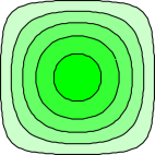
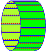
| There exist pointy vectors, which are relatively familiar to most people. They can be represented by an arrow with a tip and a tail. | There exist one-forms, which are relatively less familiar to most people. They can be represented by contour-lines, or by stacks of fish-scales as in figure 2. |
Pointy vectors and one-forms show up in a wide variety of contexts. They are given a variety of different names, and can be visualized in a variety of different ways, as tabulated near the end of item 11.
As we shall see, pointy vectors and one-forms have quite a few properties in common, since they all obey the vector-space axioms. On the other hand, there are also some crucial differences between pointy vectors and one-forms, so we have to be careful. Item 13 discusses one of the differences you need to watch out for.
| df(x1, x2, ⋯) = |
| [dxi] |
| ⎪ ⎪ ⎪ ⎪ |
| (2) |
where in the ith term of the sum, the partial derivative holds constant all the arguments to f() except for the xi argument. The notation for this is clumsy, but the idea is important. The partial derivative is really a directional derivative in a direction specified by holding constant an entire set of variables except for one … so it is crucial to know the entire set, not just the one variable that is nominally being differentiated with respect to. For details on this, including ways to visualize what it means, see reference 1.
An example is shown in figure 3. The intensity of the shading depicts the height of the function F := sin(x1)sin(x2) while the contour-lines depict the exterior derivative dF.
| (3) |
which is convenient. It simplifies the notation.
Technically speaking, [dx1] exists by fiat, according to item 2, while dx1 is something you can calculate according to equation 2. On a day-to-day basis you don’t care about the distinction, but it would have been cheating to assume they are equal. We needed to keep them conceptually distinct just long enough to prove they are numerically equal.
Suppose we want to visualize the slope of some landscape. If you visualize the slope as a pointy vector, i.e. a gradient vector it points uphill. In many cases, though, you are better off visualizing the slope as a one-form, corresponding to contour lines that run across the slope.
You can judge the magnitude of the 1-form according to how closely packed the contour lines are. Closely-packed contours represent a large-magnitude 1-form. To say the same thing the other way, the spacing between contours is inversely related to the magnitude of the one-form.
Contour lines have the wonderful property that they behave properly under a change of coordinates: if you take a landscape such as the one in figure 3 and stretch it horizontally (keeping the altitudes the same) as shown in figure 4, the slopes become less. The contour lines on the corresponding topographic map spread out by the same stretch factor, as they should, to represent the lesser slope. In contrast, if you try to represent the slope by pointy vectors, the representation is completely broken by a change in coordinates. As you stretch the map, position vectors and displacement vectors get longer, meaning they have greater magnitude, whereas slope vectors get smaller in magnitude. Therefore we need different representations. We represent positions and displacements using pointy vectors, but we represent slopes using 1-forms.
To say the same thing the other way, representing a slope using a pointy vector would be a bad idea; such vectors would not behave properly. They would not be “attached” to the landscape the way contour lines are.
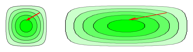
Of course, pointy vectors are needed also; they are appropriate for representing the location of one point relative to another in this landscape. These location vectors do stretch as they should when we stretch the map. An example of this is shown in red in figure 4.
It is important to clearly distinguish the two types of vector. The distinction shows up in a variety of different contexts:
| Type of vector: | pointy vector | one-form | ||
| In linear algebra: | column vector | row vector | ||
| In relativity: | contravariant vector | covariant vector | ||
| In quantum mechanics: | Dirac ket: |⋯⟩ | Dirac bra: ⟨⋯| | ||
| On a map: | displacement | gradient | ||
| Stretching the map: | increases distance | decreases steepness |
If not all the rows in that table are familiar to you, don’t worry about it.
- The difference between two position-vectors is called a separation-vector or equivalently a displacement-vector.
- A position-vector depends on the choice of origin, but a displacement-vector does not.
- The magnitude of a displacement-vector is called the distance. The distance is a scalar, not a vector.
- The magnitude of a slope is called the steepness.
Consider the contrast:
| In some spaces, we have a metric. That is, we have a dot product. That allows us to determine the length of a vector, and to determine the angle between two vectors. In such a space, we have a geometry (not just a topology). Ordinary Cartesian (x,y,z) space is a familiar example. | There are other spaces where we do not have a metric. We do not have a dot product. We do not have any notion of angle or length or distance. We have a topology, but not a geometry. Thermodynamic state-space is an important example. We can measure the distance (in units of S) between contours of constant S, but we cannot compare that to any distance in any other direction. |
| You were probably taught that a dot product is “defined” by multiplying corresponding components. That’s not the definition. It’s true sometimes, but not always. |
| In plain Cartesian x,y,z space, the distance s is given by: | On the surface of a sphere, where the vector components are latitude λ and longitude ϕ, the distance s is given by: |
| The Cartesian metric tells us the Cartesian dot product is simple. | The geodetic metric tells us the geodetic dot product is nontrivial. Near the poles a large change in longitude doesn’t mean much in terms of distance. |
| If we have a metric, we can use it to convert a row vector to the corresponding column vector and vice versa. That gives us a one-to-one correspondence: For any pointy vector you can find a corresponding one-form and vice versa. | In a non-metric space, there is not any way of converting 1-forms to pointy vectors or vice versa. There is not any way of finding a 1-form that uniquely “corresponds” to a given pointy vector or vice versa. |
| If we have a trivial Cartesian metric, the components of the row vector are numerically equal to the components of the corresponding column vector. | In general, the components are not numerically equal. You have to use the metric to find the numerical value of the components. |
| Technically, the row vectors always live in their own space, while the column vectors always live in another space. |
| Given a metric, the two spaces are isomorphic, and people usually don’t bother to distinguish them. | Without a metric, the two spaces remain distinct. It makes sense to visualize dE as a one-form, i.e. as contours of constant E ... but it does not make sense to visualize dE as any kind of pointy vector. It makes even less sense to visualize dE as any kind of scalar, infinitesimal or otherwise. E is a scalar, but the slope of E (i.e. dE) is a one-form. |
A 1-form has a direction, but we cannot measure the angle between two such directions. You can say that we have a topology but not a geometry. This sounds like a terrible limitation, but it is actually the right thing for thermodynamics, because typically you have no way of knowing whether dS is “perpendicular” to dV or not, and it causes all sorts of trouble if you use a mathematical formalism that assumes you can measure angles when you can’t.
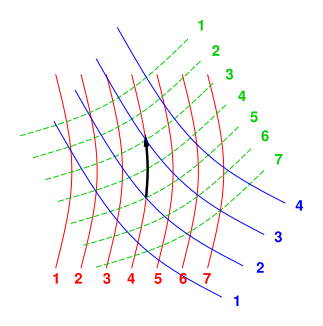
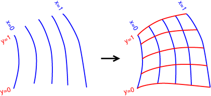
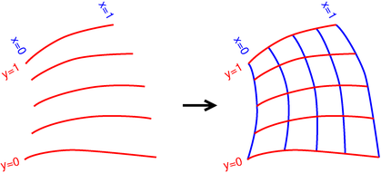
Among other things, this means that we do not require the coordinates x1, x2, ⋯ to be mutually perpendicular. Since there is no notion of distance or angle, so we could not make them perpendicular even if we wanted to. See figure 5.
| dxi ∧ dxj = −dxj ∧ dxi (6) |
for all (i, j).
Non-grady force fields are common in the real world. See reference 2 for more about how to visualize such things.
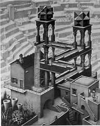
A conspicuously ungrady form w is shown in figure 6. You can imagine that this represents the 1-form w := PdV (aka “work”) in a slightly-idealized heat engine. The direction of the 1-form (i.e. the uphill direction) is everywhere counterclockwise. This w is a perfectly fine 1-form, but you cannot write w = dW because w cannot be the slope of any potential W. The concept of slope is locally well-defined, and you can integrate the slope along a particular path from A to B, but you cannot use this integral to define a potential difference W(B) − W(A) because the result depends very much on which path you choose. This is like Escher’s famous “Waterfall” shown in figure 7.
To repeat: You are free to write w = PdV. That is a perfectly fine 1-form, well-defined at every point in the state space. In contrast, it is not OK to write w = dW or PdV = dW, because that cannot be well-defined throughout state space, except perhaps in trivial cases. (You might be able to define something like that on a one-dimensional subspace, along a particular path through the system, but then you would need to decorate “W” with all sorts of subscripts to indicate exactly which subspace you are talking about.)
A more subtle example of an ungrady form is discussed in item 24 below.
| d(A ∧ B) = dA ∧ B + (−1)k A ∧ dB (7) |
where A has grade=k.
| dd = 0 (8) |
This important result can be expressed in words: “the boundary of any boundary is zero”.
Before we explain why this is so, we should emphasize that dd is not the most general second-derivative operator. Rather, it is the antisymmetric part of the second derivative, in accordance with equation 7. So what we are saying is that the antisymmetric part of the second derivative vanishes.
- By way of contrast, the symmetric part would be the familiar Laplacian ∇·∇, but that only makes sense if we have a well-defined dot product, which is not generally the case in thermodynamics.
- As another type of contrast, d applied to a scalar function is the most general first derivative, namely the slope, even though dd is not the most general second derivative.
The antisymmetric piece of the second derivative necessarily vanishes, because of the mathematically-guaranteed symmetry of mixed partial derivatives:
|
| f ≡ |
|
| f (9) |
This is true for all f, assuming f is sufficiently differentiable, so that the indicated derivatives exist.
Figure 8 and Figure 9 show what’s going on. We will use these figures to discuss finite steps (as indicated by Δ) instead of infinitesimals, but the same ideas apply in the limit of very small steps. In particular, Δx|y means to take a step toward increasing x along a contour of constant y. Similarly Δy|x means to take a step toward increasing y along a contour of constant x.
In accordance with the usual operator-precedence rules, the interpretation of the LHS of equation 9 is:
|
| f means | ⎛ ⎜ ⎜ ⎝ |
| ⎛ ⎜ ⎜ ⎝ |
| (f) | ⎞ ⎟ ⎟ ⎠ | ⎞ ⎟ ⎟ ⎠ | (10) |
That is, we work from right to left, first taking a step toward increasing y along a contour of constant x, then taking a step toward increasing x along a contour of constant y. For example, in the figure, this would correspond to proceeding clockwise from (0,0) via (0,1) to (1,1).
Meanwhile, the RHS of equation 9 tells us to proceed counterclockwise in the figure, from (0,0) via (1,0) to (1,1). The point is that we get to same point either way. That is, the clockwise trip we just took, together with the counterclockwise trip, form a “closed” figure.
This result is nontrivial. Although the boundary of a boundary is zero, the boundary of “something else” is not necessarily zero. For example:
| (11) |
Forms that are closed, including figure 3 and figure 10, have the property that the “contour” lines in one region mesh nicely with the lines in adjacent regions. In a non-closed form such as figure 6, the meshing fails somewhere. (Commonly it fails everywhere.)
Beware that this notion of “closed one-form” is not equivalent to the notion of “closed set” (containing its limit points) nor to the notion of “closed manifold” (compact without boundary). See reference 3 and reference 4.
| ∫ |
| dF = F(B) − F(A) (12) |
The meaning is simple: the integral measures the number of contours that you cross in going from point A to point B. For a grady 1-form, this number is independent of the path you take along the way from A to B.
This integral is, of course, a linear operator.
| B = fi(x) dxi (13) |
We are using the Einstein summation convention, i.e. implied summation over repeated indices, such as index i in this equation.
As explained in section 2, the integral of this is:
| (14) |