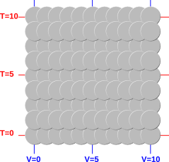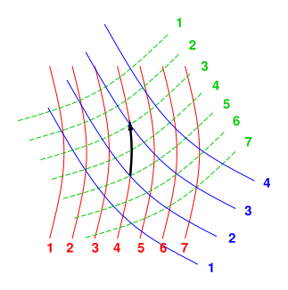
Figure 1: Contours of Constant Value (for three different variables)
You should probably start by reading reference 1, which explains some of the ideas that will be used here, including how to visualize a slope in terms of contour lines, and how to visualize it as a one-form, which is a special type of vector.
In thermodynamics, it is common to see equations of the form
where E is the energy, T is the temperature, and S is the entropy. In this example, P is the pressure, and V is the volume.
We shall see that the best approach is to interpret the d symbol as the derivative operator.2 Specifically, dS is a vector representing the slope of S. We shall explore various ways of visualizing a slope... and also ways of visualizing something like TdS that is a vector but normally not the derivative of any function. (See reference 3 for details on this.)
Note the contrast:
| The first law of thermodynamics states that energy is conserved. That’s it; nothing more and nothing less. It’s a profound statement about physics. | Equation 1 does not express conservation of energy. It’s a true statement, but it doesn’t tell us anything about physics, as discussed below. |
In particular, Equation 1a is just a reminder of what the notation means. On the next line, Equation 1b is just math. It’s the chain rule for the derivative of vectors, valid whenever E can be expressed as a differentiable function of S and V. On the last line, equation 1c is more notation. It expresses a choice, not a fundamental law. It reflects our chosen definitions of T and P, chosen to make equation 1c synonymous with equation 1b. It can be shown that these definitions agree with long-established customary notions of temperature and pressure, which is reassuring.
If, hypothetically, S were the only relevant variable, you could think of ΔS as a small change in S, and not worry about it too much.
However, in real-life thermodynamics, you could easily have 10 different variables with 7 constraints, so we are dealing with a 3-dimensional subspace of a larger space. That means you can’t change S without changing at least 6 other things at the same time. So the question arises, which other things?
Here’s the key fundamental concept: Consider making a small move to a new point in the abstract, high-dimensional state space. Then consider what happens to S as a consequence of that move. The change in S will depend on the direction of the move. The vector dS tells us everything we need to know about how S is affected by a small move in any direction in thermodynamic state space.
Again: The thermodynamic state of the system is described by a point in some abstract D-dimensional space, which is a subspace of an even higher-dimensional space, because we have more than D variables that we are interested in. Figure 1 portrays a two-dimensional space (D=2), with three variables.
You can usually choose D variables to form a linearly-independent basis set, but you don’t have to. All the variables are still perfectly good variables, even if they are not linearly independent. There are various constraints due to the equation of state, conservation laws, boundary conditions, or whatever.
Note that figure 1 does not show any axes. This is 100% intentional. There is no red axis, green axis, or blue axis; instead there are contours of constant value for the red variable, the green variable, and the blue variable. For more about the importance of such contours, and the unimportance of axes, see reference 4. The so-called red axis would point in the so-called direction of increasing value of the red variable, but in fact there are many directions in which the red variable increases.
In such a situation, if we stay away from singularities, there is no important distinction between “independent” variables and “dependent” variables. Some people say you are free to choose any set of D nonsingular variables and designate them as your “independent” variables. However, usually that’s not worth the trouble, and – as we shall see shortly – it is more convenient and more logical to forget about “independent” versus “dependent” and treat all variables on the same footing.
Singularities can occur in various ways. A familiar example can be found in the middle of a phase transition, such as an ice/water mixture. In a diagram such as figure 1, a typical symptom would be contour lines running together, i.e. the spacing between lines going to zero somewhere.
See reference 5 for an overview of the laws of thermodynamics. Many of the key results in thermodynamics can be nicely formulated using expressions involving the d operator, such as equation 1.
In order to make sense of thermodynamics, we need to answer some basic questions about dE, dS, T dS, etc.:
It turns out that the best way to think about such things is in terms of vectors – not the familiar pointy vectors but another kind of vectors, namely one-forms. The relationship between pointy vectors and one-forms is discussed in reference 1. Some suggestions for how to visualize non-grady vector fields are presented in reference 3. Additional suggestions for how to visualize partial derivatives are presented in reference 6.
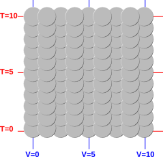
Before we get into details, let’s look at some examples. Consider some gas in a piston. The number of moles of gas remains fixed. We can use the variables S and V to specify where we are in the state space of the system. (Other variables work fine, too, but let’s use those for now.)
Figure 2 shows dV as a function of state. (See reference 5 for what we mean by “function of state”.) Obviously dV is a rather simple one-form. It is in fact a constant everywhere. It denotes a uniform slope up to the right of the diagram. Contours of constant V run vertically in the diagram.
Similarly, figure 3 shows dT as a function of state. This, too, is constant everywhere. It indicates a uniform slope up toward the top of the page. Contours of constant T run left-to-right in the diagram.
Note that the diagram of dT is also a diagram of dE, because for an ideal gas, E is just proportional to T.
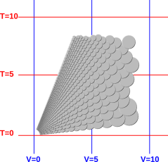
Things get more interesting in figure 4, which shows dP as a function of state. (We temporarily assume we are dealing with an ideal gas.) Since dP is the slope of something, we call it a grady one-form, in accordance with the definition given in reference 1. We can see that dP is not a constant. It gets very steep when the temperature is high and/or the gas is squeezed into a small volume. For an ideal gas, the contours of constant P are rays through the origin. For a non-ideal gas, the figure would be qualitatively similar but would differ in details.
The one-forms dS, dT, dV, and dP are all grady one-forms, so you can integrate them without specifying the path along which the integral is taken. The answer depends on the limits of integration, i.e. the endpoints of the path, not on the details of the path. When these variables take on the values implied by figure 4, you can integrate them “by eye” by counting steps. You can see that T is large along the top of the diagram, V is large along the right edge, and P is large when the temperature is high and/or the volume is small.
Tangential remark: If the following doesn’t mean anything to you, don’t worry about it. This can be formalized as follows: dS is the exterior derivative of S. dS and TdS can each be called a differential form, in particular a one-form, which is a type of vector. For the next level of detail on this, see reference 1, reference 7, and reference 8. If you want yet more detail, there exist detailed, rigorous books on the topic of differential topology. However, you don’t need to know any of this. Basic notions of slopes and partial derivatives suffice for present purposes.
Here’s a point that is just a technicality now, but will be important later: These diagrams are meant to portray the one-forms directly. They portray the corresponding scalars T, V, and P only indirectly.
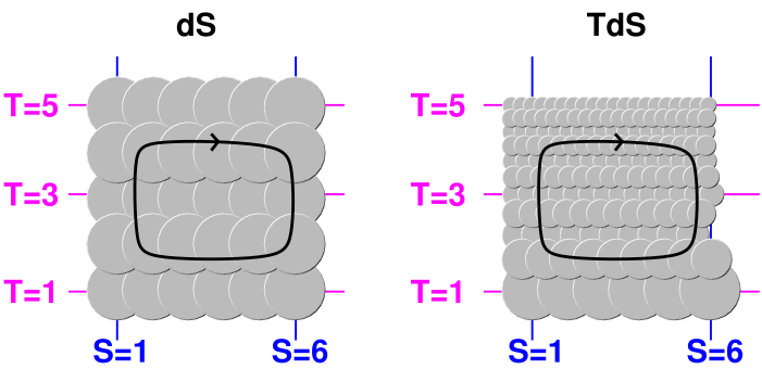
Figure 5 shows the difference between a grady one-form and an ungrady one-form.
| As you can see in on the left side of the figure, the quantity dS is grady. If you integrate clockwise around the loop as shown, the net number of upward steps is zero. This is related to the fact that we can assign an unambiguous height (S) to each point in (T,S) space. | In contrast, as you can see on the right side of the diagram, the quantity TdS is not grady. If you integrate clockwise around the loop as shown, there are considerably more upward steps than downward steps. There is no hope of assigning a height “Q” to points in (T,S) space. |
Be warned that in the mathematical literature, what we are calling ungrady one-forms are called “inexact” one-forms. The two terms are entirely synonymous. A one-form is called “exact” if and only if it is the derivative of something. We avoid the terms “exact” and “inexact” because they are too easily misunderstood. In particular:
- In this context, exact is not even remotely the same as accurate.
- In this context, inexact is not even remotely the same as inaccurate.
- In this context, inexact does not mean “plus or minus something”.
- In this context, exact just means grady. An exact one-form is the derivative of some potential.
Pedagogical remark and suggestion: The idea of representing one-forms in terms of overlapping “fish scales” is not restricted to drawings. It is possible to arrange napkins or playing-cards in a loop such that each one is tucked below the next in clockwise order. This provides a useful hands-on model of an inexact one-form. Counting “steps up” minus “steps down” along a path is a model of integrating along the path.
You may be wondering what is the relationship between the boldface d operator as seen in equation 1 and the plain old lightface d that appears in the corresponding equation in your grandfather’s thermo book:
| (2) |
The answer goes like this: Traditionally, dE has been called a “differential” and interpreted as a small change in E resulting from some unspecified small step in state space. It’s hard to think of dE as being a function at all, let alone a function of state, because the step is arbitrary. The magnitude and direction of the step are unspecified.
In contrast, dE is to be interpreted as a machine that says: If you give me an input vector ΔX that precisely specifies the direction and magnitude of a step in state space, I’ll give you the resulting change in E. In equation 1 the input vector is not yet specified, so the change in E is not yet specified – that doesn’t mean that the machine is vague or ill-defined. The machine itself is a completely well-defined function of state.
By way of analogy: An ordinary matrix M is a machine that says: If you give me an input vector ΔX, I will give you an output vector O, namely O=(M ΔX). When talking about M, we have several choices:
This analogy is very tight. Indeed, at every point in state space, dE can be represented by non-square matrix. In the example we have been considering, the state of the system is assumed to be known as a function of D=4 variables (S and the three components of X) so the slope will be a matrix one row and four columns.
Terminology: We are treating the state of the system (X) as a column vector with D-components, or equivalently as a D×1 matrix. We are treating the slope of a scalar (such as dE) as a row vector with D components, or equivalently as a 1×D matrix.
Operationally, you can (as far as I know) improve every equation in thermodynamics by replacing d with d. That is, we are replacing the idea of “infinitesimal” with the idea of one-form. To say the same thing in slightly different words: we are shifting attention away from the output of the machine (d) onto the machine itself (d). This has several advantages and no known disadvantages. The main advantage is that we have replaced a vague thing with a non-vague thing. The machine dE is a function of state, as are the other machines dP, dS, et cetera. We can draw pictures of them.
Any legitimate equation involving d has a corresponding legitimate equation involving d. Of course, if you start with a bogus equation and replace d with d, it’s still bogus, as discussed in section 3. The formalism of differential forms may make the pre-existing errors more obvious, but you mustn’t blame it for causing the errors. Detecting an error is not the same as causing an error.
The notion of grady versus ungrady is not quite the same in the two formalisms: It makes perfect sense to talk about grady and ungrady one-forms. In contrast, as mentioned in section 2.3, it’s hard to talk about an ungrady differential, since if it’s ungrady, it’s not a differential at all, i.e. it’s not the slope of anything.
Let’s forget about thermo for a moment, and let’s forget about one-forms. Let’s talk about plain old vector fields. In particular, imagine pressure as a function of position in (x,y,z) space. The pressure gradient is a vector field. I hope you agree that this vector field is perfectly well defined. There is a perfectly real pressure-gradient vector at each (x,y,z) point.
A troublemaker might try to argue that “the vector is merely a list of three numbers whose numerical values depend on the choice of basis, so the vector is really uncertain, not unique.” That’s a bogus argument. That’s not how we think of the physics. As explained in reference 9, we think of a physical vector as being more real than its components. The vector is a machine which, given a basis, will tell you the numerical values of its components. The components are non-unique, because they depend on the basis, but we attach physical reality to the vector, not the components. The vector exists unto itself, independent of whatever basis (if any!) you choose.
The pressure gradient is a vector field. As discussed in reference 1, there are two different kinds of vectors, namely row vectors and column vectors. They are not equivalent, but in simple situations the distinction doesn’t matter, in which case there are two possible ways of representing the pressure gradient:
Given a simple Cartesian metric, in any basis the three numbers representing the pointy vector are numerically equal to the three numbers representing the one-form. In simple cases there is a one-to-one correspondence between a column vector and the corresponding row vector.
Returning to thermo: Let’s not leave behind all our physical and geometrical intuition when we start doing thermo. Thermo is weird, but it’s not so weird that we have to forget everything we know about vectors. However, we have to be careful about a couple of things. In particular, there is generally not any way to construct a one-to-one correspondence between a column vector and a row vector. Both types of vectors exist, but they exist in separate vector spaces.
One-forms are vectors. They are as real as the more-familiar pointy vectors. To say the same thing another way, row vectors are just as real as column vectors.
If you think the pressure gradient dP is real and well-defined when P is a function of (x,y,z) you should think it is just as real and just as well-defined when P is a function of (V,T). Gradients (in thermo and otherwise) can always be considered row vectors, i.e. one-forms. In non-thermodynamic (x,y,z) space you have the option of also treating the slope as a column vector, i.e. a gradient vector, but in thermodynamic (T,V) space you don’t. That’s the only tricky thing about slopes in thermodynamic state space: they are row vectors only.
Let us briefly consider taking a finite step (as opposed to an infinitesimal differential). The definition of ΔE is:
| ΔE := EA − EB (3) |
where B is the initial state A is the final state. That is, A stands for After and B stands for Before.
Before we can even consider expanding ΔE in terms of PΔV or whatever, we need to decide what kind of thing ΔE is.
Since E is a scalar, clearly ΔE is a scalar. Also, it has the same dimensions as E. As always, we assume E is a function of state. So far so good.
The problem is, ΔE is not a function of state. Equation 3 tells us ΔE is a function of two states, namely state A and state B.
Let’s see if we can remedy this problem. First we perform a simple change of variable. Rather than using the two points A and B, we will use the single point (A+B)/2 and the direction A−B. That is, we say the Δ(⋯) operator pertains to a step centered at (A+B)/2 and oriented in the A−B direction. This notion becomes precise if we take the limit as A approaches B. We now have something that is a function of state, the single state (A+B)/2 ... but it is no longer a scalar, since it involves a direction.
At this point we have essentially reinvented the exterior derivative dE. Whereas ΔE was a scalar function of two states, dE is a vector function of a single state.
Let’s review, by looking at some examples. Assuming the system is sufficiently well behaved that it has a well-defined temperature:
| (4) |
You may be accustomed to thinking of dS as the “limit” of ΔS, in the limit of a really small Δ ... but it must be emphasized that that is not the modern approach. You are much better off interpreting the symbols as follows:
These two itemized points are related: Changing the ordinate from scalar to vector is necessary, if we want to change the the abscissa from two states to a single state.
In addition to nice expressions such as equation 1, we all-too-often see dreadful expressions such as
| (5) |
As will be explained below, T dS is a perfectly fine one-form, but it is not a grady one-form, and therefore it cannot possibly equal dQ or d(anything), assuming we are talking about uncramped thermodynamics.
Note: Cramped thermodynamics is so severely restricted that it is impossible to describe a heat engine. Specifically, in a cramped situation there cannot be any thermodynamic cycles (or if there are, the area inside the “cycle” is zero). If you wish to write something like equation 5 and intend it to apply to cramped thermodynamics, you must make the restrictions explicit; otherwise it will be highly misleading.
The same goes for P dV and many similar quantities that show up in thermodynamics. They cannot possibly equal d(anything) ... assuming we are talking about uncramped thermodynamics.
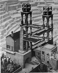
Trying to find Q such that T dS would equal dQ is equivalent to trying to find the height of the water in an Escher waterfall, as shown in figure 6. It just can’t be done.
Of course, T dS does exist. You can call it “almost” anything you like, but you can’t call it dQ or d(anything). If you want to integrate T dS along some path, you must specify the precise path.
Again: P dV makes perfect sense as an ungrady one-form, but trying to write it as dW is tantamount to saying
«There is no such thing as a W function, but if it did exist, and if it happened to be differentiable, then its derivative would equal P dV.»
What a load of double-talk! Yuuuck! This has been called a crime against the laws of mathematics (reference 10).
Constructive suggestion: If you are reading a book that uses dW and dQ, you can repair it using the following procedures:
As for the idea that T dS > T dStransferred for an irreversible process, we cannot accept that at face value. For one thing, we would have problems at negative temperatures. We can fix that by getting rid of the T on both sides of the equation. Another problem is that according to the modern interpretation of the symbols, dS is a vector, and it is not possible to define a “greater-than” relation involving vectors. That is to say, vectors are not well ordered. We can fix this by integrating. The relevant equation is:
| (6) |
where we integrate along some definite path Γ. We need Γ to specify the “forward in time” direction of the transformation; otherwise the inequality wouldn’t mean anything. It is an inequality, not an equality, because it applies to an irreversible process.
At the end of the day, we find that the assertion that «T dS is greater than dQ» is just a complicated and defective way of saying that the irreversible process created some entropy from scratch.
Note: The underlying idea is that for an irreversible process, entropy is not conserved, so we don’t have continuity of flow. Therefore the classical approach was a bad idea to begin with, because it tried to define entropy in terms of heat divided by temperature, and tried to define heat in terms of flow. That was a bad idea on practical grounds and pedagogical grounds, in the case where entropy is being created from scratch rather than flowing. It was a bad idea on conceptual grounds, even before it was expressed using symbols such as dQ that don’t make sense on mathematical grounds.
Beware: The classical thermo books are inconsistent. Even within a single book, even within a single chapter, sometimes they use dQ to mean the entire T dS and sometimes only the T dStransferred.