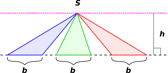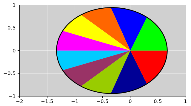
Figure 1: Kepler’s Equal-Area Law
We will discuss various ways of explaining Kepler’s equal-area law, and its connection to angular momentum. We will also mention other familiar and not-so-familiar conserved quantities, such as the energy and the Laplace-Runge-Lenz vector.
We will also show that the usual “geometric” proof of the equal-area law is a swindle. It assumes that the average force is equal to the instantaneous force, which is not only unproven, but provably untrue in the situation shown in the usual diagram. If you are going to argue that the error goes away in the limit, you have to actually make the argument. You have to exhibit the error, and prove not only that it decreases, but that it decreases to zero fast enough.
Kepler’s equal-area law states that the radius vector from the sun to a planet sweeps out equal areas in equal times. This is also known as Kepler’s second law. It was published in 1609. The idea is illustrated in figure 1. Each of the ten colored sectors has the same area.
The way this works is that when the planet is close to the sun it moves faster. When it is far from the sun it moves slower.
The spreadsheet used to calculate all the orbit diagrams in this document is cited in reference 2.
There is a widely-known formula that says the area of a triangle is equal to half of its base times its height. You get to pick one side of the triangle and call it the base. Then the height – also known as the altitude – is the projection of the triangle onto the direction perpendicular to the base. You can easily rederive this result if you want: Arrange two copies of the triangle to make a parallelogram, then slice and re-arrange the parallelogram to make a rectangle.
In particular, each of the triangles in figure 2 has an area of ½bh, since each has base b and height h.
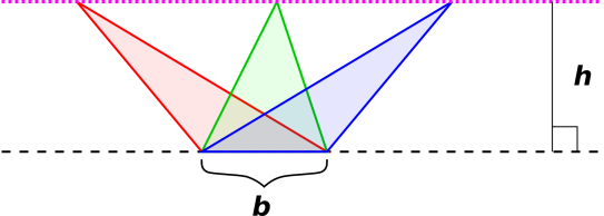
There is another way to construct a series of triangles with equal area. Whereas figure 2 keeps the apex of the triangle fixed at point S and moves the base, you can equally well leave the base fixed and move the apex along a line parallel to the base, such as the dotted magenta line in figure 3. Either way, so long as the height is unchanged and the length of the base is unchanged, the area will stay the same.
We can connect this to physics as follows: Suppose we have a free particle moving through empty space. In accordance with the first law of motion, it moves in a straight line with uniform velocity v. Let’s suppose its path coincides with the dashed black line near the bottom of figure 2. Every time the particle encounters one of the triangles, it will take the same amount of time to cross from one side of the base to the other. The crossing time is b/|v|.
To say the same thing another way: The radius vector from S to the particle will sweep out equal areas in equal times. This is a simple example of Kepler’s second law, as mentioned in section 1.
In the context of a free particle, there is nothing special about the point S. You can choose any point in the universe, and you will find that the particle’s angular momentum about the chosen point is conserved.
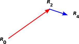
Now suppose we have a particle that is only “mostly” free. That is, most of the time it moves freely, moving in a straight line with uniform velocity. However, every so often, it gets hit with a hammer. We approximate each hit as an impulse, i.e. an instantaneous transfer of momentum. This is associated with a sudden change in the velocity of the particle. The trajectory of this particle is illustrated in figure 4.
The figure shows three points, R0, R2, and R4. The points are abstract points, with no size, no direction, or anything else.
Without loss of generality, we assume that the three labeled points in figure 4 are equally spaced in time. Therefore the displacement vectors connecting successive points are proportional to the velocity vector associated with that segment of the path.
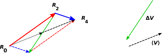
We could analyze this system using algebra and Cartesian coordinates if desired, but let’s do something else instead. We can analyze it using classical geometric techniques. Let’s start by using the parallelogram rule to construct the sum and difference of the velocities. This is shown in figure 5.
The green diameter of the parallelogram is the difference (blue velocity minus red velocity) which we denote by ΔV. The full black diameter from R0 to R4 is the sum. Half the sum is the average, which we denote by ⟨V⟩. The average is indicated by the dashed black vector or (equivalently) the dotted black vector.
| The next step involves constructing another parallelogram. As we do this, keep in mind that a vector has direction and magnitude ... but not a position. That means we can copy a vector and/or move it around, so long as we don’t change its direction or magnitude. |
In
situations involving angular momentum, we care about the force vector
and its point of application. If you choose an origin, the vector from the origin to the point of application is called the lever arm. We then have two vectors: The force has direction and magnitude, and separately the lever-arm has direction and magnitude. |
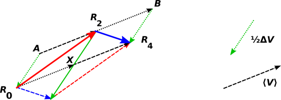
We use these ideas to describe an imaginary secondary particle that approaches point R2 at the average velocity ⟨V⟩ and then departs at the same velocity. This is shown in figure 6.
| The dotted green vectors that go from A to R0 and from B to R4 are equal to ½ΔV. It must be emphasized that they do not represent an impulse applied at the point R0 or R4. Indeed, they are just vectors, devoid of any notion of point of application. We moved them into position to facilitate applying the parallelogram rule. | To describe the impulse, we need both a vector (with direction and magnitude, as shown by the solid green vector) and a point of application (such as R2). |
The parallelogram AR2XR0 illustrates the mathematical fact that the red velocity is equal to the average minus half of the delta. Similarly, the parallelogram BR4XR2 illustrates the fact that the blue velocity is equal to the average plus half of the delta.
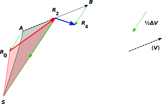
This allows us to obtain an interesting result: consider the red-shaded triangle and the gray-shaded triange in figure 7. They have equal area, because they share the same base and have equal height. Note that as the apex moves from B to R4, it moves along a line parallel to the applied impulse, i.e. parallel to ΔV.
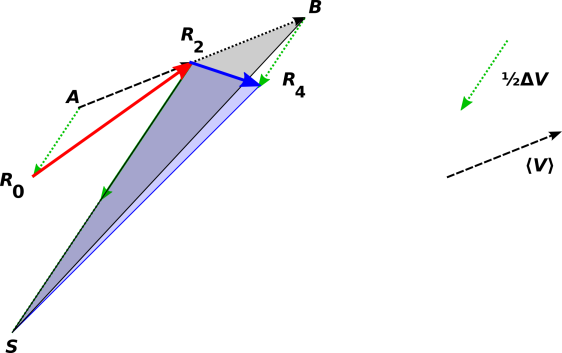
Similar words could be said about the blue and gray triangles in figure 8. They have equal areas. This is an application of the sliding-apex lemma mentioned in section 2.
What’s more, both of the gray-shaded triangles have the same area. This is an application of the sliding-base lemma mentioned in section 2.
By the transitive property of equality, we now know that all four of the shaded triangles are equal in area. The two we care most about are the red-shaded and blue-shaded triangles, since they tell us about the actual trajectory of our particle. They tell us that the particle sweeps out equal areas in equal times. In other words, the motion of our particle is consistent with constant angular momentum about S. We should not be surprised by this, because the applied force has zero lever arm about S.
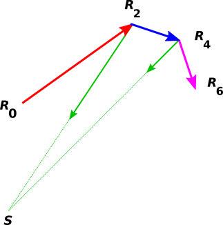
So far we have considered only one impulse, which means the point S could be chosen anywhere along the line passing through R2 in the direction of the applied impulse. In other words, it could be chosen anywhere that gives zero lever-arm to the applied impulse. However, the story changes if we have more than one impulse.
| Newton’s law of universal gravitation as applied to point particles is a central force. | For extended objects, not so much. The earth exchanges angular momentum with the moon, via gravitational effects. This is not a first-order effect, but rather a higher-order (i.e. tidal) effect. |
We begin this section with a heuristic argument that goes like this:
To the extent that these approximations are valid, this suggests that continuous motion in a central force-field will have constant angular momentum.
Let’s be clear about what we have proved and not proved:
| We have outlined a classical geometrical proof of the fact that for an intermittent, impulsive, central force, angular momentum about the center is constant. Kepler’s equal-area law is upheld. | We have a heuristic argument but not a proof of the corresponding result for a continuous central force. |
Heuristic arguments are useful. In particular, a heuristic argument might motivate you to look for a proof, and might guide the design of the proof.
On the other hand, it is bad luck to prove things that are not true. A heuristic argument must not be passed off as a proof. If something is true “in the limit” but not otherwise, you should not claim to have proved it in the non-limiting case.
It’s also bad luck to assume things that are not true. For the Kepler problem, the approximations enumerated above are definitely only approximations. They are not exact in the non-limiting case. Let’s try to understand why not.
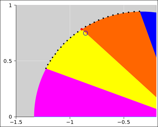
We shall be interested in the point of application of the forces. Figure 10 is a close-up of the ellipse shown in figure 1. The black dots represent points along the ellipse, equally spaced in time. The midpoint in time is highlighted in red. The unfilled blue circle represents the average of these points, averaged over two adjacent sectors as shown.
Note the contrast: If you average the times for these 25 points and find the position corresponding to that time, you get the red dot. However, if you average the 25 positions directly, you get the blue circle. In other words, the time-averaged position is not equal to the instananeous position. This means that approximation #1 as given above is only an approximation. It might converge to the exact answer “in the limit” but otherwise it’s not exact.
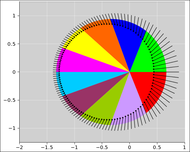
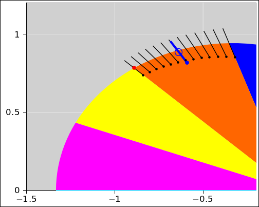
We shall also be interested in the magnitude and direction of the forces. Figure 11 shows the orbit and also the forces at various points. Each instantaneous force vector is represented by a black arrow. You can see that when the orbit is near the sun, the forces are larger, in proportion to 1/r2, in accordance with Newton’s law of universal gravitation. You can also see that each of the forces is directed toward the sun, again in accordance with Newton’s law of universal gravitation.
The black arrows in figure 11 are doing double duty: The midpoint of each black arrow is colocated with the point of application. (This sort of double duty can sometimes be used to simplify a diagram, but it should be used with caution, because it blurs the concept of point-of-application with the concept of direction-and-magnitude.)
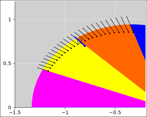
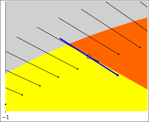
We can average the vectors, averaging over two sectors, to get the average vector shown in blue in figure 12. The point of application is wrong, as already discussed, and furthermore the force itself is wrong as to direction and magnitude. It’s not off by much, but it is definitely off, as you can see in the close-up in figure 13. In other words, the time-averaged force is not equal to the instantaneous force. That means approximation #2 as given above is only an approximation. It might converge to the exact answer “in the limit” but otherwise it’s not exact.
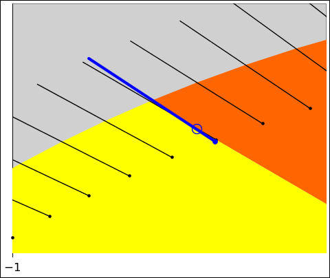
Figure 14 shows the same situation as figure 13. The only1 difference is that we have relocated the blue vector so you can more easily compare it to the nearby black vector. You can see that difference in magnitudes is rather small, while the difference in directions is not quite so small. 2
From this we conclude that we are nowhere near having a high-school geometry-style proof of Kepler’s equal-area law. Maybe such a proof exists, but I have never seen any such thing. The idea of limits belongs to calculus, not to high-school geometry. This situation is part of what motivated Newton to invent calculus. See however section 5.5.
Limits are a tool. Like any tool, they can be used properly or improperly. In particular, simply increasing the number of edges on a polygon is nowhere near sufficient to guarantee that the approximations enumerated above converge to the right answer. For example, for a sufficiently unsteady central force, the time-averaged force at the corners of the polygon might never converge to the instantaneous force. Similarly, for a sufficiently non-smooth path, the instantaneous position at the corners might never converge to the time-averaged position.
Here’s how the tool can go wrong: Suppose there is a smallish error, such as we see in figure 11 or figure 13. As we increase the number of sides on the polygon, making each side smaller, the error gets smaller ... but that’s not good enough! The problem is, there are more sides and therefore more errors. A large number of small errors might add up to a big problem. To make the limit work, you have to prove that the errors get small fast enough, sufficiently fast that even when you add them up, the total gets smaller and smaller, and indeed goes to zero as we pass to the limit. To repeat:
Therefore we cannot accept the argument given in reference 3. It purports to prove using polygons that the result holds for any central force. First of all: If you are making an argument that depends on taking the limit, you have to actually say that. Then you have to actually do the work to show that the total error goes to zero. Now it turns out that using calculus ideas you can prove that the actual 1/r2 force field is sufficiently well behaved, and you can prove that the actual path of the planet is sufficiently well behaved. Still, you have to actually do the work to prove that; you can’t just tacitly assume it.
It’s also wrong to suggest that high-school geometry methods suffice to prove the general result for an arbitrary central force-field and an arbitrary trajectory. If you mean to restrict the result to some kind of well-behaved force-fields and well-behaved trajectories, you have to actually say that.
Most importantly: As a general rule, keep in mind that a diagram is not a proof. A diagram might help explain a proof, and a diagram might even help you discover a method of proof, but you still need to do the proof. This is the biggest problem with the diagram in reference 3 and the corresponding diagram in reference 4. The diagrams assume without proof, without evidence, and without explanation that the instantaneous force is equal to the average force. They use the same vector with two different meanings. Sure, you can draw a diagram where the average force-vector is pointing in the same direction as the instantaneous force, but that doesn’t make it true. In fact we know it’s not true except in the limit. It’s not true for any real polygon with sides of nonzero size. Any such diagram is a swindle. The only honest thing to do is to draw the diagram with enough detail to show that the average force is merely “close” to the instantaneous force ... and then do the work necessary to show that the error goes to zero fast enough to make the limit converge.
Let’s summarize the status of the proposition that the instantaneous force is equal to the average force:
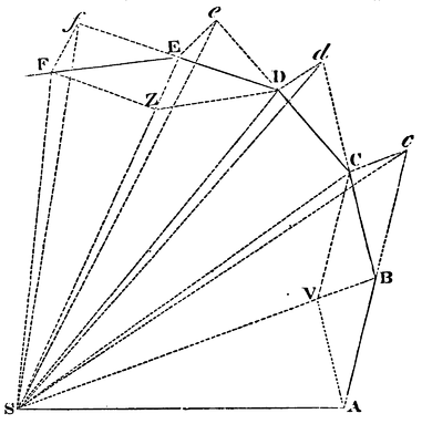
Calculus does not appear in the Principia. Based on unpublished papers and other sources we know that Newton invented calculus long before writing the Principia, but he chose not to present it in the book. Instead he relied on geometrical arguments of the type we have been discussing. The diagram he used in connection with the equal-area proposition is reproduced in figure 15. I cannot say why this is. Perhaps Newton himself did not fully trust the new methods, or perhaps he trusted them but did not think his readers would understand and/or trust them.
Either way, Newton has thrown the baby out with the bathwater. He has relieved the reader from the small burden of reading about limits, but saddled the reader with the much larger burden of re-inventing limits. To say the same thing in more detail: The geometrical approach is either not correct or (at best) not applicable to real planets. Therefore the reader must (a) notice that Newton’s diagram and proof only work for polygonal paths, (b) figure out that to apply the idea to real life, a limit must be performed, and (c) re-invent the rules for taking limits.
Figure 6 is symmetrical about the point R2 in the sense that it treats the past and future on the same footing. As we said before, it illustrates the twin mathematical facts that the red velocity is equal to the average minus half of the delta, and the blue velocity is equal to the average plus half of the delta.
You could equally well do the arithmetic in a less-symmetrical way. If you do it entirely to the left of point R2, it says the red velocity is equal to the blue velocity minus the delta (the full delta, not half). If you do it entirely to the right of point R2, it says the blue velocity is equal to the red velocity plus the delta. The latter is how it is done in reference 4 and reference 3. This bit of vector arithmetic has the same meaning in all of these arrangements.
As a minor point, I find figure 6 to be more elegant, because it is more symmetrical. However, that is not the real issue.
A much more significant advantage to figure 6 is that it explicitly constructs the average as well as the delta, whereas the diagrams in reference 4 and reference 3 only construct the delta. If you don’t construct the average, you are skipping a crucial step in the argument when it comes time to argue that the polygon is an approximation to the ellipse.
Another significant advantage to the symmetrical approach is discussed in section 5.7.
Once you decide to construct the average position and average force, there are significant advantages to doing it in a symmetrical way. From the point of view of a purely mathematical theoretical proof, proving that the average values converge to the instantaneous values, there is not much advantage, because the lopsided averages do converge eventually. However, in practical numerical calculations, where you are actually using a polynomial to approximate the orbit, “eventually” isn’t the only thing you care about. The convergence is much quicker if you calculate the averages in a nice symmetrical way.
You can see in figure 16 that if we take a lopsided average, the average position (blue circle) is nowhere near the instantaneous position (red dot). It is a much worse approximation than what we saw in figure 12. Similarly, you can see in figure 17 that the average force is a much worse approximation to the instantaneous force than what we saw in figure 13. Again we have relocated the average vector. This facilitates comparison to the instantaneous vector.
Such considerations are beyond the scope of high-school geometry. They come under the heading of “numerical methods”. Using sound numerical methods can improve the efficiency and accuracy by orders of magnitude. In some applications, this can make the difference between succcess and failure.
A fairly comprehensive summary of the equations applicable to Keplerian orbits can be found in reference 5. Beware that the mass of the orbiting particle is implicitly assumed to be unity. This is a common practice, and makes sense because the mass drops out of the astronomically-observable kinematic variables, in accordance with Einstein’s principle of equivalence. Some additional equations can be found in reference 6. The symbols are a bit nonstandard, but the standard names are given, so it is possible to decode things. Yet more equations can be found in reference 7.
In the context of orbital mechanics, the fundamental gravitational law is conventionally written as
| (1) |
where m is the mass of the orbiting particle and the constant κ (kappa) combines the universal gravitational constant and the mass of the attracting object, and k = κ m. The object is assumed to be infinitely massive compared to the orbiting particle.
It is common practice to speak of a “central” force and to call the attracting object the “central” object. However, note that if the attracting object is not infinitely massive compared to the orbiting object, then both objects orbit around a common center. So, it is at best risky to talk about a “central” object. It is still OK to speak of the center of the force field. However, even then, beware that the center of the force field is not at the center of the ellipse, but rather at one focus. So if you talk about “the” center, you have to be clear about which center you are talking about.
The total energy is a constant of the motion, namely:
| (2) |
where a is the semi-major axis of the orbit. Combining equation 2 with equation 1 gives us useful expressions for the kinetic energy and speed:
| (3) |
Kepler’s second law says that the areal velocity is a constant.
| (4) |
where θ is the azimuthal angle as seen from the attracting body, also known as the true anomaly; π a b is the total area of the ellipse; upper-case P is the period; and lower-case p is the momentum. The semi-minor axis, the semi-minor axis, and the eccentricity are related via:
| (5) |
We are particularly interested in the “mean anomaly” M and its rate of change, namely:
| (6) |
Also:
| (7) |
The next step toward finding the position is to plug M into Kepler’s equation, i.e.:
| (8) |
where Æ is the eccentric anomaly. It is commonly denoted E, but we call it Æ to avoid conflicting with the energy. Reference 8 discusses the problem of solving Kepler’s equation for Æ in terms of M. It’s a transcendental equation, and no closed-form expression for the inverse equation is known. The spreadsheet in reference 2 uses a few iterations of Newton’s root-finding algorithm.
The components of the position-vector can be rather simply expressed in terms of Æ:
| (9) |
We can obtain the components of the velocity by differentiating the position:
| (10) |
The speed calculated in this way can be compared with the speed calculated from energy considerations (equation 3), which gives us a sensitive check on the calculations.
To use equation 10 we need Æ·, which we can find by differentiating Kepler’s equation:
| (11) |
That may look like another transcendental equation, but since we have already solved for Æ it’s really just a simple algebraic equation that can easily be solved for Æ·.
Let us temporarily restrict attention to the Kepler problem, i.e. a 1/r2 force field. It is conventional (but not entirely wise) to define the Laplace-Runge-Lenz vector as follows:
| (12) |
Here r⊥ is the projection of r onto the direction perpendicular to the instantaneous momentum (or, equivalently, to the instantaneous velocity). That is:
| (13) |
In equation 12, the forms without cross products (using only dot products) are strongly preferred, because they are well defined in any number of dimensions from two on up, whereas the cross product is only defined in three dimensions. Besides, the cross product involves a right-hand rule, and it seems silly to involve any notion of handedness in a system where the fundamental physics is left/right symmetric.
The quantity (r × p) is the angular-momentum pseudovector. We are always better off avoiding that, and instead thinking of the angular momentum as a bivector:
| (14) |
This allows us to avoid all the silliness associated with cross products. See reference 9 for an explanation of bivectors, wedge products, et cetera. In particular, we are better off replacing equation 12 with the following:
| (15) |
Equation 14 and equation 15 work fine in all dimensions from two on up.
The name eccentricity vector is applied to a scaled version of the LRL vector:
| (16) |
Using the 1/r2 force law, (equation 1), we can rewrite the last term on the RHS of equation 15:
| (17) |
For the Kepler problem, this vector A is conserved. This quantity is not nearly so familiar as energy or angular momentum, but it is nevertheless conserved. In the spreadsheet (reference 2), calculating A from the definition and checking that it is constant provides another sensitive check on the numerical accuracy of the calculations.
If we expand our field of view to include any central force law, there are two choices.
For more on this, see reference 10.