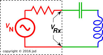
Figure 1: Series RLC Circuit, Grounded Capacitor
Consider the RLC circuit in figure 1. There are at least two ways of thinking about it.
We start by applying Ohm’s law for complex impedances in series. The input to the filter is V0 which we will set equal to VN. The phasor current is:
| (1) |
Note that the reactive parts of the impedance add to zero at the corner frequency. (In contrast, for a parallel RLC circuit, the reactive parts would combine in parallel to make an infinite impedance at the corner frequency.)
At the moment we are not interested in the phase, so we focus attention on the magnitude of the current. Compare eq 12.3.8 in reference 1.
| (2) |
The magnitude of voltage across the capacitor is:
| (3) |
where
| (4) |
Note that 1/RC has dimensions of frequency. This has important but non-obvious physical significance, as discussed in section 1.6.
The corner frequency is the intersection of the asymptotes. The true resonant frequency, as defined by the position of the peak, is not quite the same, although it converges to the corner frequency in the high-Q limit. See equation 14 and equation 28.
The magnitude of the gain squared is:
| (5) |
where δ is the R/L bandwidth:
| (6) |
This gives us one possible notion of bandwidth. See section 1.6 for a discussion of this and other frequency-like quantities.
The quality factor Q can be expressed in a variety of useful forms:
| (7) |
and the reactive reference impedance is:
| (8) |
We can equally well write things in terms of the circular (not angular) frequency. Circular frequency can be measured in units of hertz (not radians per second). That gives us:
| (9) |
We can also write things in terms of the normalized frequency. We define:
| (10) |
whereupon:
| (11) |
Continuing down the road toward more streamlined expressions, we can write things in terms of frequency squared. We define:
| (12) |
whereupon:
|
where the key parameters of the resonator are:
| (14) |
Equation 13c and equation 14 were obtained by completing the square. Note that in equation 13c (unlike in previous expressions), the first term in the denominator in a constant, independent of frequency.
In the context of spectroscopy, equation 13c is called a Lorentzian. In particular, it is a Lorentzian function of the square of the frequency. I’m not quite sure why it’s called that. In the context of probability, the same function is called a Cauchy distribution. Furthermore, it’s essentially the same function as the “Witch” of Agnesi, and Agnesi has more than 100 years priority. On top of all that, Fermat studied the same function 100 years before Agnesi. Evidently this is yet another example of Stigler’s law of epononymy.
Expressing it in standard Lorentzian form makes it easy to pick off the abscissa and ordinate of the peak.
To find the FWHM, we set
| (15) |
and solve for frequency squared:
| (16) |
which reduces to 2/Q in the high-Q limit.
However, we are mainly interested in the frequency ϕ (not frequency squared), so we write
| (17) |
which reduces to 1/Q in the high-Q limit. More generally:
|
where
| (19) |
When Q is equal to Qmin, the height of the peak is 2. For smaller Q values, the concept of a “peak” with a “FWHM” goes out the window. You can still define a notion of “width” but the meaning is different.
Not coincidentally, the radius of convergence of the Taylor series in equation 18c is 1/Q = 1/Qmin.
Consider the Nyquist formula for the Johnson noise source inside a resistor. It should be written as:
| (20) |
where the brackets ⟨⋯⟩ denote the ensemble average. This is the voltage of the ideal noise source, deep inside the black box, where it is not directly observable. The real resistor consists of everything inside the black box in figure 1, i.e. the noise source plus the ideal noiseless resistance. The externally observable voltage VRx at the terminals of the black box depends on the noise source and on the IR voltage drop across the ideal resistance.
All too often the formula is written in the less-careful form:
| (21) |
where it requires some care to figure out what is meant by V and what is meant by the bandwidth B. If you apply equation 21 incautiously, you might imagine that you need is B, not the gain or the area under the curve. However, as usual, it pays to think about where the formula comes from. Since we are interested in the voltage on the capacitor (not just the resistor), I claim the actual physics says:
| (22) |
integrated over circular (not angular) frequency. Now in some ideal world where the ideal noise source is driving a filter such that the voltage gain G is unity within a passband of width B and zero everywhere else, then equation 22 reduces to equation 21. However, in the other 99.999999% of the cases, you actually have to do the integral. Figure out what’s happening at each frequency, and then add up all the contributions.
As a warm-up exercise, we calculate the area under the gain-squared curve, without worrying about the input voltage:
| (23) |
The whole idea of gain means if we know the square of the input voltage, we can multiply by the square of the gain (at any given frequency) to find the square of the output voltage, i.e. the voltage across the capacitor.
We now apply this to the special case where the input voltage is thermal noise, so the input is given by equation 20. We multiply by gain squared, and sum over all frequencies:
| (24) |
The average energy in the capacitor is:
| (25) |
as expected, as required by thermodynamics, as required by fundamental notions of equipartition. The result is independent of Q, resonant frequency, and everything else. The calculations leading up to equation 25 may seem like a complicated way of obtaining a simple and familiar result, but they are worth the trouble, because they provide a powerful check on the calculations up to this point.
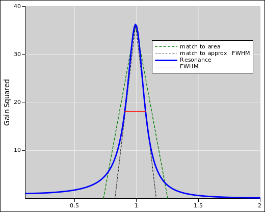
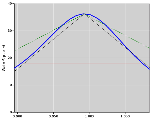
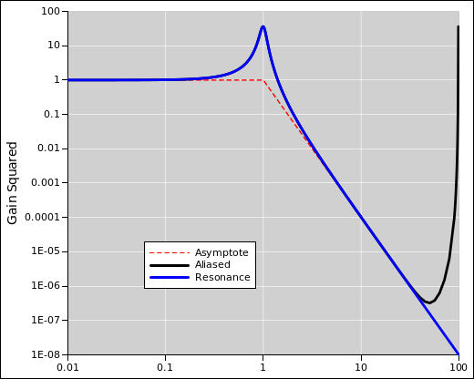
Of course, the mean-square voltage and average energy are not the only things that you can measure. You can also hook up a spectrum analyzer and measure things as a function of frequency. The results should look like figure 2 and figure 4.
In any frequency bin from a to b, the mean square voltage in that bin is:
| (26) |
but you might have to worry about aliasing, as discussed in section 3.2.
Suppose our friend Simplicio looks in a book and finds that «the» bandwidth of an RLC oscillator is B = R/L, and then uses that as the B in equation 21. At this point he has already made three mistakes:
Combining this with the previous item gives a factor of Q2/(2π).
Combining this with the previous items gives us an overall factor of Q2/4. So the effective noise bandwidth is not R/L but rather 1/(4RC), which is what we see in equation 23.
To repeat: When the Q is not too small, you can approximate the lineshape as a triangle. Note the contrast:
| To get the right height and the right area, use a triangle with a height of Q2, a width (i.e. FWHM) of (π/2) (f0/Q), and an area of (π/2) Q f0. This is indicated by the dotted line in figure 2. Alas this doesn’t match the FWHM very well. | If you leave out the factor of π/2 and simply set the FWHM to f0/Q, you get a much better match to the FWHM. This is indicated by the dotted line in figure 2. Alas, this seriously underestimates the area. |
| The discrepancy between the two triangles leads to holy wars about the definition of “the” width. Increasing the Q does not make the discrepancy go away; there is always considerable weight in the wings of the distribution. This is unlike a Gaussian, where there is not much weight in the wings, and you can match it with a triangle with the right area and the right FWHM within a few percent, as discussed in reference 2. |
Another possible pitfall is aliasing, as discussed in section 3.2.
At the corner frequency the height is:
| (27) |
If Q is not very high, the actual peak of the resonance is slightly taller than that, and occurs at a slightly lower frequency; see equation 14 and equation 28.
Also note:
In addition to equation 13, here is another way of locating the peak. Set the derivative of (gain squared) to zero. Then:
| (28) |
At that frequency, the height of the peak is as follows, as you can verify by direct substitution:
| (29) |
Both equation 28 and equation 29 agree with the results we obtained in equation 14 by other means.
The following figures were made using the spreadsheet mentioned in reference 3.
| (30) |
| (31) |
| (32) |
It has dimensions of frequency, but it is not what people think of as the bandwidth of the resonance. It could be considered the effective noise bandwidth, if we were rash enough to interpret equation 24 as 4 kT R times some bandwidth, and ignore a factor of 4, and ignore the issue of gain.
A better way to think of 1/(RC) is as a bandwidth times gain squared. The RLC circuit doesn’t just “select” the components of the incoming signal that lie within the passband; it also amplifies those components.
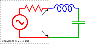
There are at least five voltages of interest in our circuit:
This is closely analogous to the analysis in section 1.1.
| (33) |
The magnitude of voltage across the capacitor is:
so the magnitude of the gain is:
|
where as before:
| (36) |
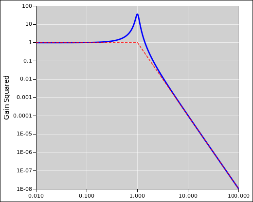
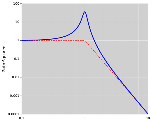
Equation 35 says the gain goes to unity at high frequencies. This should be obvious from looking at the circuit diagram. At the resonant frequency, the height of the peak is Q.
We now turn to the “digital signal processing” point of view. That is, we imagine the current, voltage, etc. are represented by time-series data, i.e. a sequence of samples.
This stands in contrast to section 1, which analyzed things from an analog point of view.
Let the time between samples be Δt.
The thermal noise source, internal to the resistor, should have a mean square voltage:
| (37) |
where fN is the Nyquist frequency. Compare equation 21.
Here’s one way to understand why fN appears in this expression: Imagine this noise source is driving a filter, and ask how big much bandwidth B is needed in order to capture all of the power coming from this source. That is the meaning of the B used in the derivation of the Nyquist formula.
You can verify that this is correct as follows: Use this voltage to drive a filter. An ultra-simple RC filter suffices. Integrate the equations of motion numerically. Verify that the average thermal energy in the capacitor is ½ kT, independent of all circuit parameters.
The RLC filter responds to waves at negative frequencies just as well as to positive frequencies. That means it looks like the black curve in figure 7. At the Nyquist frequency it is a factor of 2 higher than the blue curve (which is the same as in figure 4). One octave below the Nyquist frequency, it is higher by a few percent.
In this example, the sampling rate is 200 Hz, so the Nyquist frequency is 100 Hz. On linear axes the curve is symmetrical, i.e. an even function of frequency, but the symmetry is lost when we plot it on log axes.
When fitting the data, if you’re in a hurry you might just throw away the top two octaves ... but it’s almost as easy to include the aliasing in the model. Instead of equation 9, use the following:
| (38) |
where g is the sampling frequency minus f. At the Nyquist frequency, g=f.
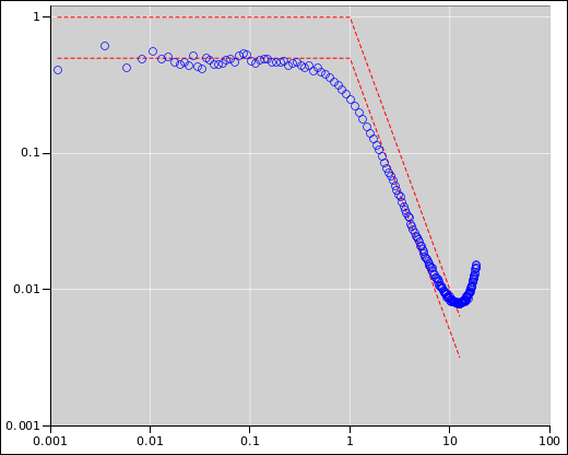
Here is some real data, from timestepping the equations of motion for a simple RC (not RLC) circuit. That can be done super-easily.
The corner frequency is 1 Hz, and the Nyquist frequency is 12.5 Hz. The ordinates are normalized to the ideal intrinsic noise in the resistor, so they “should” go to one at low frequency, because the filter has unity gain at low frequencies. The power-spectrum data as reported by the FFT, as shown in the figure, is off by a factor of two, because of aliasing. Half of the energy we are looking for is lurking at negative frequencies. When we look at the FFT we see only positive frequencies, whereas a real hardware RC has no such restriction.
As long as the resonant frequency is small compared to the Nyquist frequency, and you don’t look too closely at the tails of the distribution (as discussed in section 3.2), the results should be independent of the sampling rate.
In practice, digitial filters are always followed by analog filters, to solve the aliasing problem.
In our case, the RLC makes a fine analog filter all by itself, and (if properly used) will filter out 99.99% of the ugliness at negative frequencies and high frequencies.