Figure 1: Small Rotations
Abstract: It is well known in physics – and even in pop culture – that time is the fourth dimension. Obviously the time dimension (t) is not exactly the same as the other three (x, y, and z), but it is more closely analogous than many people realize. The tx plane has a geometry and even a trigonometry, just as the xy plane does. For example, what would be called a slope in the xy plane is called a velocity when it occurs in the tx plane. The relativistic addition-of-velocities rule is nonlinear for the same reason that slope is a nonlinear function of angle: it’s just trigonometry. Leveraging our understanding of the xy plane makes it easy to understand the essential features of special relativity, including the fact that no object can be accelerated to the speed of light, and the fact that the speed of light is the same in all reference frames.The geometry of spacetime is remarkably similar to the geometry of ordinary space, with just one salient difference. This can be understood at many levels. In this paper, we focus on the simplest levels, using pictures, vectors, and a little bit of trigonometry. (In reference 1, we re-explain and validate the ideas using a more formal approach.)
Additional Keywords: rotation/boost; angle/rapidity; slope/velocity; correspondence principle; hyperbolic trigonometry; gorm.
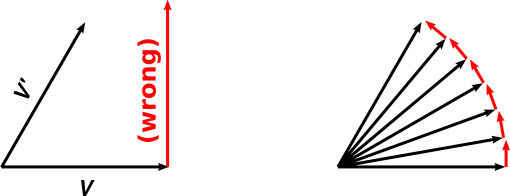
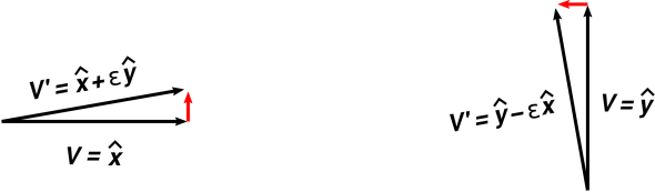
We assume the reader has a basic understanding of what it means to rotate something in the xy plane. It is, however, worth reviewing some of the basic ideas, to establish the notation and to lay the foundation for further developments. We begin by examining the effect of a small xy rotation, such as is shown in figure 1.
We start with a vector V pointing in the x̂ direction, as shown on the left side of figure 1. We rotate it by an angle є to form another vector V’. When є is small, the difference vector (V’ − V) is very nearly perpendicular to V. The difference vector is shown in red in the figure. We can express the effect of the rotation as:
| (1) |
If instead we start with a vector pointing in the ŷ direction, as shown on the right side of figure 1, the effect is very similar: rotation causes the vector to pick up a component in a perpendicular direction. For our chosen direction of rotation, the new component is in the negative x direction:
| (2) |
Rotating a sum of vectors is the same as rotating each of the summands separately. Since any vector in the xy plane can be written as a linear combination of x̂ and ŷ, we can rotate any vector simply by combining equation 1 and equation 2. The overall effect is:
| (3) |
When we consider larger rotations, it is not satisfactory to plug in a larger value of є in these equations (perhaps as shown on the left side of figure 2). Instead, we break the large rotation into a sequence of small rotations – all in the xy plane – each of which is well described by equation 3, as shown on the right side of the figure.
If you do the math, combining N rotations each of size є = θ/N, you get one overall rotation of size θ. In the limit of large N, the overall rotation can be expressed in the familiar form:
| (4) |
If this expression for V’ is not familiar, a helpful exercise is to set q=1 and r=0 and evaluate this expression for various values of θ from zero to 360∘ in steps of 30∘. Plot the resulting V’ vectors.
It is easy to see that equation 3 is a consequence of equation 4, by considering what happens when θ becomes very small. (If that’s not obvious, you can verify it by evaluating cos(θ) and sin(θ) for small values of θ using a calculator. Make sure the calculator accepts θ in radians.) It is also straightforward to prove the converse, namely that equation 4 is necessarily and uniquely the result of applying equation 3 N times ... but we defer the proof to reference 1.
We introduce the idea of boost by saying a small boost is just a small change in velocity ... which is something we already understand in terms of basic physics. Let’s see if we can parlay our understanding of small boosts into an understanding of large boosts, by treating boosts the same way we treated rotations in the previous section. A good discussion of boosts, with much additional detail, can be found in reference 2. A more advanced discussion, including a electromagnetic fields in spacetime, can be found in the early chapters of reference 3.
We start by plotting the position of a particle as a function of time. Such a plot is familiar from high-school physics. We choose to call it by a slightly fancy name, namely the world line of the particle, plotted on a spacetime diagram. Note that we plot the t axis vertically, as is conventional in the field of relativity. This has several advantages, including the fact that the x axis is horizontal in both figure 3 and figure 1. (Beware that this conflicts with the convention commonly used in introductory physics, which plots motion as x versus t with the t axis horizontal.)
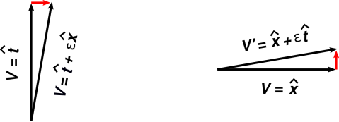
For starters, let’s consider a particle at rest in our reference frame. If we take a step along the world line of the particle, the t coordinate changes, but the x coordinate does not. We can represent this act – stepping along the world line – by a vector that points in the t̂ direction, such as the vector V on the left side of figure 3.
Next consider a second particle that is moving with a small velocity relative to the first particle. (We say it has been boosted by an amount є in the tx plane.) If we take a step along this particle’s world line, the t coordinate changes in the usual way, but we also pick up a slight change in the x coordinate, as shown by the vector V’ on the left side of figure 3. Such a step can be represented by a vector of the form t + є x. The boost operation itself can be represented as:
| (5) |
We emphasize that up to this point, we have done nothing subtle or tricky. We take a step in the V’ direction along the particle’s world line. It has a certain slope, a certain Δ x over Δ t. This is just velocity. This is just prosaic high-school physics.
The units in equation 5 bear some explaining. As a preliminary step, we choose to measure distance in meters and measure time in jiffies, where a jiffy is the time it takes for light to travel one meter. In these units, c=1 meter per jiffy. As the next step, we take to heart the profound correspondence between space and time, and decide that a jiffy just another name for a meter; specifically, a meter of extent in the timelike direction. As the final step, we drop the distinction between ordinary meters (spacelike meters) and jiffies (timelike meters). In these units, c=1. For the same reason, є is dimensionless in equation 5, just as it was in equation 1.
Remark: This is the first subtle step in the derivation. It is not obvious from nonrelativistic mechanics what value to use for c. For now we can consider it an arbitrary conversion factor from spacelike units to timelike units. Later we can ascertain that c must be the speed of light. This can come from the Michelson-Morley experiment, or perhaps from an examination of the Maxwell equations; details are beyond the scope of this document.
Presumably you have noticed that equation 5 and equation 1 have essentially the same form and the same meaning. That is to say, a boost in the x dirextion is just a rotation in the xt plane. Our discussion of rotations in the xt plane will be very nearly but not quite identical to the previous discussion of rotations in the xy plane.
It turns out that if you take a vector in the x̂ direction and boost it in the tx plane, the result is as shown on the right side of figure 3. It can be expressed as:
| (6) |
Remark: The plus sign in equation 6 stands in contrast to the minus sign in equation 2. This is the second – and last – subtle step in the whole discussion. This seemingly-innocuous change of sign has the most profound consequences, as will be discussed in section 5.
But first, we should finish working out the general formula for boosts. Boosting a sum of vectors is the same as boosting each of the summands separately, so we can combine equation 5 and equation 6 as follows:
| (7) |
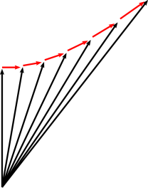
To understand a large boost, we break it into a sequence of small boosts – all in the tx plane – each of which is well described by equation 7, as shown in figure 4.
If you do the math, combining N boosts each of size є = ρ/N, you get one overall boost of size ρ. In the limit of large N, the overall boost can be expressed in the form:
| (8) |
It is easy to see that equation 7 is a consequence of equation 8, by considering what happens when ρ becomes very small. (If that’s not obvious, you can verify it by evaluating cosh(ρ) and sinh(ρ) for small values of ρ using a calculator. Some students might benefit from making a graph of the cosh() and sinh() functions, perhaps by hand or perhaps by means of a spreadsheet.) It is also straightforward to prove the converse, namely that equation 8 is necessarily and uniquely the result of applying equation 7 N times ... but we defer the proof to reference 1.
Remark: In the relativity literature, the symbol β has long been used to represent the quantity tanh(ρ); see e.g. reference 4. Similarly, γ is used to represent cosh(ρ).
Consider the following contrast:
| – spacelike rotations – | – timelike rotations – |
| A rotation in a spacelike direction is sometimes called a twist. | A rotation in a timelike direction is sometimes called a boost. The angle of rotation is sometimes called the rapidity. |
| The idea of angle is particularly useful, because a sequence of rotations of sizes θ1, θ2, θ3 – all in the yx plane – has the same effect as one big rotation of size θ, where θ = θ1 + θ2 + θ3. | The idea of rapidity is particularly useful, because a sequence of boosts of sizes ρ1, ρ2, ρ3 – all in the tx plane – has the same effect as one big boost of size ρ, where ρ = ρ1 + ρ2 + ρ3. |
| Sometimes we are interested in the slope, which is equal to tan(θ). Note that slope does not have the additivity property mentioned in the previous paragraph, except when the slope is very small. For instance, figure 2 can be thought of as six wedges piled on top of each other, tip atop tip. The top of the first wedge has a slope of 1 part in 6, but that does not mean that six wedges combine to make a 1:1 slope. In fact they make a slope that is more than 1.5:1, quite a bit more than a linear extrapolation would have predicted. As you add more wedges, the slope grows more and more quickly. Soon it passes through infinity and becomes negative. | Sometimes we are interested in the classical velocity, i.e. the reduced velocity, which is equal to tanh(ρ). Note that velocity does not have the additivity property mentioned in the previous paragraph, except when the velocity is very small. For instance, figure 4 can be thought of as a sequence of six boosts: Each particle in the sequence is moving relative to the previous one with a speed of 1/6th of the speed of light, but that does not mean that particle #6 is moving relative to particle #0 at 100% of the speed of light. In fact, the combined velocity is only 76% of the speed of light, quite a bit less than a linear extrapolation would have predicted. As you make more and more such boosts, the combined velocity keeps growing more and more slowly. It asymptotically approaches the speed of light. |
| The locus of the arrowheads in figure 2 is a circle. It is the result of rotating a given vector V by various amounts. | The locus of the arrowheads in figure 4 is a hyperbola; see reference 5. It is the result of boosting a given vector V by various amounts. |
Not coincidentally, the coefficients appearing in equation 4
are circular trig functions:
|
Not coincidentally, the coefficients appearing in equation 4
are hyperbolic trig functions:
|
In previous sections, we have considered multiple vectors (notably V and V’) using only one frame of reference. We now wish to change viewpoints, and henceforth consider only one vector at a time, using multiple frames of reference (notably the “red” and “blue” frames). This is sometimes called using passive transformations, in contrast to the previous active transformations. The reference frames will be rotated, but the vector V will not. The basis vectors in the blue frame are t̂B, x̂B, and ŷB. Similarly, the basis vectors in the red frame are t̂R, x̂R, and ŷR.
Keep in mind that our spacetime diagrams have the t axis pointing upward, as is conventional in the field of relativity. (This is in contrast to high-school physics, where it is more common to plot the t axis horizontally. It doesn’t actually matter. You can do it either way, and the meaning is the same.)
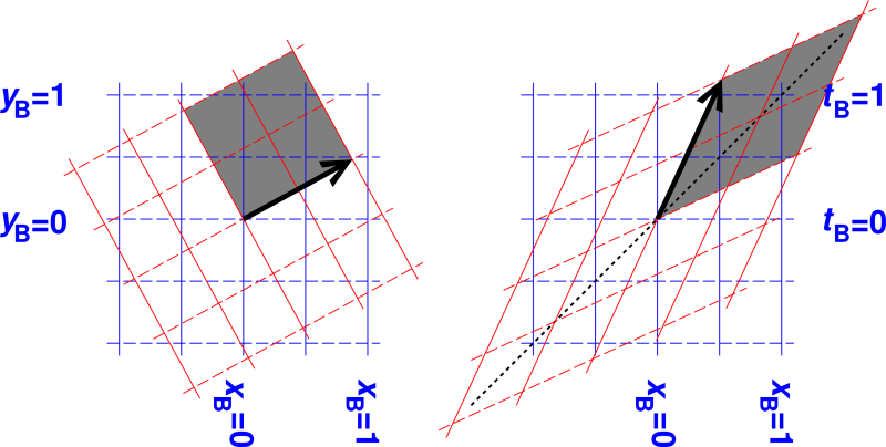
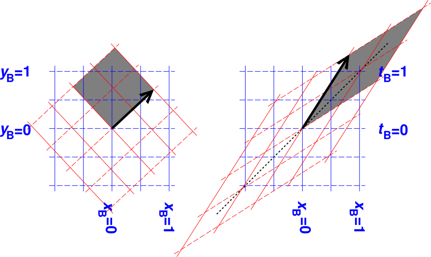
These ideas are depicted in figure 5, figure 6, and figure 7. Each figure has two diagrams, one for rotation in the xy plane (on the left) and one for rotations in the xt plane (on the right).
The lines in the diagram are drawn according to the following rules:
| constant x | constant y or t | ||||
| Blue frame: | solid blue | dashed blue | |||
| Red frame: | solid red | dashed red | |||
| The red frame is angled relative to the blue frame. In the three figures, the angle is θ=0.25, 0.50, and 0.75 radians respectively. | The red frame is moving relative to the blue frame. In the three figures, the rapidity is ρ=0.25, 0.50, and 0.75 respectively. |
| A rotation in the xy plane mixes x and y, in the following sense: | A rotation in the xt plane mixes t and x, in the following sense: |
| A vector that has only an x component in the red frame has both x and y components in the blue frame. The the rate-of-change of y with respect to x is what we call the slope. | A vector that has only a t component in the red frame has both t and x components in the blue frame. The the rate-of-change of x with respect to t is what we call the classical velocity. |
| We define the slope as m := tan(θ). (Recall that we are measuring angles in radians.) | We define the reduced velocity as v = tanh(ρ). (Recall that we are measuring velocities in units of meters per jiffy.) |
| When θ is small, tan(θ) is equal to θ to first order. That means slope is synonymous with angle, when the slope is small. | When ρ is small, tanh(ρ) is equal to ρ to first order. That means velocity is synonymous with rapidity, when the velocity is small. |
| As θ increases from zero to 90 degrees, tan(θ) starts out equal to θ but soon becomes larger – eventually very much larger than θ. This can be seen in the figures: Find the x and y components by projecting the black arrow onto the axes. As always, the slope is y per unit x. | As ρ increases from zero to very large values, the reduced velocity starts out equal to ρ, but soon becomes smaller – eventually very much smaller than ρ. This can be seen in the figures: Find the x and t components by projecting the black arrow onto the axes. As always, the reduced velocity is x per unit t. |
When the red frame is angled relative to the blue frame
by an amount θ, the components of V
in the red frame will be different from the components in
the blue frame, even though it’s the same vector.
|
When the red frame is moving relative to the blue frame,
by an amount ρ, the components of V
in the red frame will be different from the components in
the blue frame, even though it’s the same vector.
|
| for arbitrary scalars q and r. This conveys the same physics as equation 4. | for arbitrary scalars p and q. This conveys the same physics as equation 8. |
We now wish to discuss lengths and angles. We have to be careful, because a spacetime diagram is not an entirely faithful representation of spacetime. That is, we wish to describe events that take place in the tx plane, which has one spacelike dimension and one timelike dimension. When we represent this on paper, though, the paper has two spacelike dimensions. The mapping from spacetime to paper distorts the lengths and angles.
In particular, in each of the six diagrams, the gray-shaded area is a unit square. That is, edges of each gray area all have unit length, and adjacent edges are perpendicular. This is obvious in the xy plane, but somewhat less obvious in the xy planes. (Also we need to be careful what we mean by “unit" length, as discussed below.)
In all cases, it is obvious that the gray area in the red reference frame is square, since it is aligned with his axes. The gray area in the blue reference frame is also square, but to confirm this we have to do some calculations.
As always, we use the dot product to formalize and quantify our notion of lengths and angles.
The familiar dot product can be defined by postulating
|
The four-dimensional dot product can be defined by postulating
|
The dot product is commutative and distributes over addition in the usual way.
We hereby define the gorm of a vector to be the dot product of the vector with itself. If the gorm is positive, we say the vector is spacelike. If the gorm is negative, we say the vector is timelike. If the gorm is zero, we say the vector is lightlike, or equivalently null.
Let A and B be two points (i.e. events) in spacetime, and let V be the displacement vector, V := B − A. If V is spacelike, we define the chord length to be √V·V, which is also called the invariant spatial interval. If on the other hand V is timelike, we define the chord time to be √−V·V, which is also called the invariant time interval. For a null vector, the invariant interval is zero. Chord length and chord time are discussed in reference 6.
In equation 14, the minus sign in the definition of t̂·t̂ tells us that our notion of perpendicularity in spacetime will be different from the corresponding notion in ordinary space. This peculiar minus sign is necessary to be consistent with the peculiar plus sign in equation 6, and vice versa.
We say two non-null vectors are perpendicular or equivalently orthogonal if and only if their dot product is zero.
| In simple Euclidean space, only one notion of “norm” is needed, namely |V| := √V·V. The quantity V·V is simply called the norm squared. | In Minkowski space, we need to think clearly about three different quantities: the gorm, the chord time, and the chord distance. It’s not clear we should define a “norm” at all, but if we do, it must be defined differently for timelike and spacelike vectors. The gorm must not be thought of as the norm squared. |
| Beware that the literature is horribly inconsistent in its definition of “the” invariant interval, aka “the” spacetime interval, often blurring the distinction between timelike intervals and spacelike intervals. |
| The vector qx̂ + rŷ is perpendicular to rx̂ − qŷ, for any coefficients q and r, assuming both x̂ and ŷ are spacelike. | The vector pt̂ + qx̂ is perpendicular to qt̂ + px̂, for any coefficients p and q, assuming t̂ is timelike and x̂ is spacelike. |
| Among other things, this means that in figure 1, the difference vectors are perpendicular to the position vectors in accordance with equation 4. | Among other things, this means that in figure 3, the difference vectors are perpendicular to the position vectors in accordance with equation 8. |
| It also allows us to verify that on the left side of figure 5, adjacent edges of the gray square are in fact perpendicular. | It also allows us to verify that on the right side of figure 5, adjacent edges of the gray square are in fact perpendicular, even though they may not look that way at first glance. |
| In all reference frames, each edge of the gray squares has gorm equal to 1. | In all reference frames, the spacelike edge of the gray square has gorm equal to 1, while the other edge – the timelike edge – has gorm equal to -1. We call this a unit square, since -1 fits the mathematical definition of unit. |
The idea of spacetime – the idea that time is the fourth dimension – is due to Minkowski (1908). See reference 7.
The geometry of the xy plane is
determined by the coefficients in equation 3.
|
The geometry of the tx plane is determined by the coefficients in
equation 7.
|
Our attention is captured by the element in the upper-right corner, since that is the only difference between equation 15 and equation 16.
This element tells us about the so-called breakdown of simultaneity at a distance. That is, it tells us that the time-component in the red reference frame is offset relative to the time-component in the blue reference frame – offset by an amount depending on the distance (x), and also depending on how fast the red frame is moving relative to the blue frame. This is illustrated by the right half of figure 3 and quantified by equation 6.
Throughout most of history, i.e. before relativity, this contribution was assumed to be zero. Everybody tacitly assumed that timekeeping was independent of location and independent of velocity. Indeed it is very nearly independent, unless you have a combination of large distances, multiple reference frames with high relative velocity, and highly accurate timekeeping – as you can see from the structure of equation 6. It was not until the end of the 19th century that Michelson and Morley did experiments that disproved the pre-relativity assumptions.
Michelson and Morley observed that the speed of light was the same in all reference frames. The geometry of the tx plane as defined by equation 8 has exactly this property, as you can see in e.g. figure 6. The loosely-dashed diagonal line represents the speed of light. Notice how the red t axis and x axis are both tilted toward the diagonal, so that anything that lies along the diagonal in the blue frame also lies along the diagonal in the red frame.
The Michelson-Morley experiment, and innumerable others like it, are sufficient to tell us that the upper-right element in equation 16 must be +є, not zero or anything else.
Einstein said any theory should be as simple as possible, but not
simpler. We have seen that special relativity is as simple as it
possibly could be. The geometry of the tx plane is as closely
analogous to the geometry of the xy plane as it possibly could be.
The only difference is that the sign in equation 6
differs from the sign in equation 2. Virtually all of special
relativity can be seen as arising from this one little
change. Specifically:
– This is what makes spacetime different from plain old
space.
– This is what makes the timelike dimension t different from
the spacelike dimensions x, y, and z.
– This is why you cannot accelerate an object to the speed of
light or beyond.
– This is why the speed of light is the same in all reference
frames.
It is worth taking a moment to consider what would happen if the upper-right element in equation 16 were changed to a −є, thereby making a rotation in the xt plane behave the same as a rotation in the xy plane. That would make the theory very simple ... but alas too simple, because it would make the time axis just another space axis. For example, you would be able to interchange the t axis and the x axis by an ordinary rotation, and you could travel backward and forward in time just as easily as you move east and west.
In section 4, we used passive transformations. That is, in figure 6, there is one vector – only one vector – shown in black. If we switch from the blue reference frame to the red reference frame, the vector is unaffected. The vector neither knows nor cares what reference frame, if any, we are using. For background on this, see reference 8.
We did this to make the following point: According to the “geometric” approach, special relativity primarily describes the geometry of spacetime. It does not depend on anything funny happening to the vectors, clocks, rulers, odometers or other objects that inhabit spacetime. Objects are neither Lorentz contracted nor time dilated; they are completely unaffected by boosts. The components obtained by projecting a vector onto this-or-that reference frame are affected, but that is a property of the projective geometry of the situation, not a property of the vector itself. This idea and its consequences are discussed in reference 6.
As suggested in reference 2, suppose we have a spaceship. Initially it is at rest with respect to the earth. It then accelerates steadily, such that the passengers aboard the spaceship feel a constant 1G acceleration, always in the same direction. Question: At the end of one year, how fast is the spaceship going, relative to the earth?
Solution: In the first second, the spaceship picks up a velocity of v1 = 9.8 meters per second. We know this from basic physics, and the definition of 1G. This corresponds to a rapidity of ρ1 = v1/c = 3.27e-8. The rapidity-change in each second thereafter is the same, as you can verify by considering how things look in a reference frame instantaneously comoving with the spaceship. After one year (3.16e7 seconds) this adds up to ρ = 1.03, which is an amusing result in itself: one G for one year gives you about one unit of rapidity.
Since tanh(1.03) = 0.77, we conclude that the reduced velocity is 77% of the speed of light.
Our method of solution made heavy use of the additivity property discussed in section 3. This is easy to understand by analogy to ordinary spacelike rotations.
There are other ways of solving this problem, but none easier or more elegant.
It is, alas, rather time-consuming to draw the spacetime diagrams with the required accuracy. Therefore it is worth finding a way to do some of the work in advance.
A very useful first step is to prepare some “spacetime graph paper” containing two sets of axes: one set of ordinary unboosted (x,t) axes, plus another set of boosted axes, carefully drawn with the correct angles and the correct units.
Often it is remarkably easy to compute the diagrams. Many drawing programs have a way of applying an arbitrary linear transformation to a sub-image. This can be used to boost vectors, or even more complex objects. All the diagrams in this paper were computed.
Note that when we consider combinations of boosts in more than a single direction, it is provably impossible to have a full discussion of boosts without also discussing spacelike rotations. That is because it is easy to construct a sequence of boosts whose net effect is a purely spacelike rotation (with no net boost). An example of this is the Thomas precession.
To say the same thing another way, purely spacelike rotations form a subgroup of the Lorentz group, whereas boosts do not. (If you don’t know what this means, don’t worry about it.)