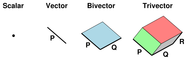
Figure 1: Scalar, Vector, Bivector, and Trivector
In this document, we discuss rotations, including simple rotations in the plane but also including compound rotations around multiple axes in three or more dimensions. We briefly survey four ways of pictorially representing rotations: two vectors in the plane of rotation, triad before and after rotation, axis plus amount of rotation, and yaw/pitch/roll. These can (respectively) be formalized in terms of (respectively) Clifford algebra i.e. quaternions, matrices, Rodrigues vectors, and Euler angles. See section 12.
Also, there is a deep relationship between ordinary rotations (in D=3 space) and boosts1 (in D=1+3 spacetime). Therefore we would like to represent rotations in a way that is consistent with special relativity. In fact Clifford algebra makes the generalization from ordinary space to spacetime as simple as it could possibly be: it suffices to change one minus sign in one equation. See section 5.
We discuss the Clifford algebra representation in some detail, because it is ideal for keeping track of rotations per se, especially if there are many different rotations to keep track of. It is elegant, it is efficient, and it is easily converted to any other representation. This has the pedagogical advantage of requiring only a small step beyond an elementary understanding of vectors. In particular, matrices are not required. (If you’re not familiar with matrices, just skip the few places in this document that mention matrices. You will still be able to represent compound rotations – including boosts – in arbitrarily-many dimensions, using Clifford algebra alone.) This representation is older than you might think, considerably older than any notion of vector cross product (reference 1, reference 2, and reference 3).
The matrix representation is particularly efficient if you have one particular rotation and wish to apply it repeatedly, using it to rotate a large number of vectors. The advantage is most conspicuous in four or more dimensions. See section 7.
Being able to deal with rotations has many practical applications. For instance, suppose you want to build an autopilot or a flight simulator. You need to be able to figure out the overall effect of a long sequence of rotations about multiple axes.
Most people, unless they are unusually well trained or unusually gifted, have a hard time visualizing rotations in D=3 or higher. For example, here’s a puzzle: suppose you apply 90 degrees of yaw followed by 90 degrees of roll. What’s the overall effect? Answer: it is a 120 degree rotation, and the plane of rotation is given by x+y+z=0. It can also be seen as a cyclic permutation of the x, y, and z axes. Most people find this puzzle somewhat discombobulating the first time they see it. See section 4.4.
This document is also available in PDF format. You may find this advantageous if your browser has trouble displaying standard HTML math symbols.
Rather than talking about the axis of rotation, we choose to emphasize the plane of rotation. This has many advantages; among other things, it works equally well in D=2 flatland, in D=3 space, in D=1+3 spacetime, et cetera. This permits unification and simplification of many ideas.
Also, once you get used to it, the plane of rotation just “looks” more natural than an axis of rotation. If you are sitting in an aircraft, you can see the plane of rotation for yaw-wise rotations spread out in front of you, running left/right. It is somewhat less natural to visualize the vertical axis (even though the two representations are technically equivalent in D=3). Similarly it is natural to think of the pitching motion as motion in a vertical plane, rather than as motion around a horizontal axis.
As we shall see below, you can encode both the plane of rotation and the amount of rotation by specifying two vectors. The plane containing the two vectors is the plane of rotation, and the angle between the two vectors tells us something about the angle of rotation; specifically, it tells us the half-angle, as will be discussed in section 2.1.
The exact choice of vectors doesn’t matter; there are many different pairs of vectors that specify the same rotation. In the language of Clifford Algebra, this means that only the product of the two vectors matters. For an introduction to Clifford algebra, and its application to geometry and physics, see reference 4, reference 5, reference 6, and reference 7.
This technique (representing a rotation as a product of vectors) is Lorentz-invariant. That is, if Alice is using a frame that is rotated relative to Bob’s frame, and also moving relative to Bob’s frame, everybody agrees as to what rotation is represented by a given product-of-vectors.
There are no singularities in the product-of-vectors representation i.e. Clifford algebra i.e. quaternions. In contrast, there are nasty singularities in the Euler angle representation, as discussed in section 12.
There is one slight quirk with the product-of-vectors representation. The angle between the vectors cannot directly represent the whole angle of rotation. To see why not, consider 180 degree rotations. If you start out heading north then apply 180 degrees of yaw, you wind up heading south, right-side up. In contrast, if you start out heading north and apply 180 degrees of pitch, you wind up facing south upside down.
The problem is that two vectors with a 180 degree angle between them are collinear, so there are many inequivalent planes that contain both vectors.
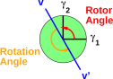
There is a simple way to fix this problem: Let the angle between the vectors represent half the angle of rotation. That is, given two vectors in the plane of rotation, we define the rotor angle to be the angle between the two vectors. The rotor represents a rotation, where the rotation angle is twice the rotor angle. Loosely speaking, we say a rotor is half of a rotation.
A 180 degree rotor represents a 360 degree rotation. For this special rotation, you don’t need to specify the plane of rotation, so the fact that these two vectors are collinear isn’t a problem. It all works out.
This half-angle business may seem like a kludge, but in fact it has a deep physical significance. One way to see the significance is in terms of reflections, as discussed in section 9.3.
In the previous section we argued on geometric and pictorial grounds that two vectors in the plane of rotation should provide a nice representation of rotations.
That leaves us with the question of how best to quantify this notion. We shall see that Clifford algebra is the perfect tool for this. Sometimes the same ideas are discussed in terms of quaternions, which correspond to a subset of Clifford algebra, as discussed in section 11.
Clifford algebra is not very complicated; it is only a few small steps beyond ordinary vector algebra. It is amazingly elegant, and is useful for many, many things, not just rotations. Since this document is focussed on rotations, this is not the place for a general tutorial on Clifford algebra. Instead we rely on reference 4 and reference 7.
To proceed, you need to appreciate the existence of scalars, vectors, and bivectors. (There also exist trivectors et cetera, although we have no immediate need of them.) You should learn to visualize such things, as in figure 1. We will explain how to form the sums and geometric products of such things.
However, to make this document at least formally self-contained, we recite here the most crucial properties of Clifford algebra. (If you want to understand the concepts the lie behind this formalism, please see the references, especially reference 4.
Suppose we can find three linearly-independent spacelike vectors. That means we must live in a space with at least three dimensions. (The generalization to any number of dimensions, from D=2 on up, is straightforward.) Applying the Gram-Schmidt algorithm to these vectors, we can construct three orthonormal vectors, namely γ1, γ2, and γ3. We do not attribute any special properties to these vectors, beyond being orthonormal and spacelike; in particular they do not need to be aligned with the cardinal directions up/down, east/west, or anything like that.
Multiplication of orthogonal vectors is anticommutative, and the product is a bivector:
| γi γj = − γj γi (bivector) (1) |
for all i ≠ j.
The product of parallel vectors is a scalar. Spacelike unit vectors are normalized like this:
| γi γi = +1 (scalar) (2) |
for all i.
Sometimes we also notice that timelike vectors exist. The timelike unit vector (γ0) is normalized differently:
| γ0 γ0 = −1 (scalar) (3) |
Clifford Algebra also defines the reverse of a product of vectors, formed by writing all the vectors in the reverse order. For example:
| (4) |
for any scalars a and b.
We can use our set of orthonormal vectors as a basis, expressing any vector in the space as a linear combination of basis vectors.
This approach – expressing everything in terms of components relative to a given basis – is definitely not the most elegant approach, and is usually not even the easiest approach, but it seems expedient in this case, for a couple of reasons: (1) Many of the illustrative examples (below) revolve around perpendicular vectors, and it’s nice to have a set of such vectors lying around. (2) Computers are good at manipulating numbers, but not so good at manipulating real physical objects like vectors and bivectors. So in computer programs, such as the one mentioned in section 13, at some point we need to project our vectors (etc.) onto a particular basis, and manipulate the components.
In contrast, if you want to see what the more-physical less-numerical approach looks like, see reference 4.
Now we are in a position to quantify the idea of using two vectors to represent the plane of rotation and the amount of rotation. In section 2 we introduced, qualitatively, the idea of rotor angle.
We now define a simple rotor to be the product of two vectors, normalized to unity (as discussed section 4.3). By product we mean the geometric product, as defined by Clifford algebra. (Non-simple rotors will be discussed in section 6.)
Note that there is a one-to-one correspondence between quaternions and a subalgebra of Clifford algebra, as discussed in section 11.)Also note that a rotor is not a bivector; in general it has a scalar piece as well as a bivector piece.
We will show that equation 5 is the completely general formula for using a rotor r to rotate a vector v. We have not yet proved or even motivated2 this result; instead we pull the formula out of thin air and then show, in retrospect, that it has the desired behavior. The key formula is:
| v′ = r∼ v r (5) |
where v is the unrotated vector, v′ is a vector that is rotated relative to v by some angle δ, and r is is a rotor with rotor angle є ≡ δ/2.
That’s all there is to it. Given two vectors in the plane of rotation, you can use them to build a rotor r. Then you can use the rotor r to perform rotations in accordance with equation 5.
Compound rotations are represented by a product of rotors in the obvious way; see section 8 and section 13 for details and reference 8 for luridly explicit details.
The simplest possible rotor is the product γ1 γ2. Since the vectors γ1 and γ2 are perpendicular, the rotor angle must be 90 degrees, and the corresponding rotation angle is 180 degrees. Let’s do the math:
| (6) |
where all we needed were the axiomatic anticommutation relations (equation 1) and the fact that multiplication is associative. Similarly we have:
| (7) |
whereas in contrast, vectors perpendicular to the γ1 γ2 plane are unaffected by the rotation:
| (8) |
and in general, for any arbitrary vector in D=3 space:
| (9) |
which is exactly the correct behavior for a 180 degree rotation in the γ1 γ2 plane. (Here a, b, and c are arbitrary scalars.) This rotation is depicted in figure 2.
It is worth emphasizing that this result is a direct consequence of the axioms of Clifford algebra, plus our decision to represent a simple rotor as a product of vectors.
If we want equation 5 to represent rotations, we must choose vectors such that their product is normalized to unity. Without this constraint, we would be inadvertently representing size-changing transformations as well as rotations. It suffices for the rotor to be a product of unit vectors, but in all generality only the product must be normalized. That is, if we have a rotor r which is the geometric product of spacelike vectors P and Q, i.e. r = PQ, it is sufficient but not necessary for the vectors P and Q to be separately normalized. All we really require is that:
| gorm(r) = 1 (10) |
where the gorm of r is, by definition, the scalar part of r∼ r. For example, the gorm of (a + b γ2 γ3) is equal to (a2 + b2), for arbitrary scalars a and b. For details, see reference 4.
Let’s return to the puzzle posed in section 1. That is, suppose you apply 90 degrees of yaw followed by 90 degrees of roll. What’s the overall effect?
We can easily compute the answer using rotors. We start with the rotor
| cos(45∘) + sin(45∘) γ2 γ3 (11) |
which we hope will represent a 45 degree rotor angle, and hence a 90 degree rotation in the γ2 γ3 plane. You can verify this by considering the product of r with itself, namely:
| (√(.5) + √(.5) γ2 γ3) (√(.5) + √(.5) γ2 γ3) = γ2 γ3 (12) |
which we recognize as the 90 degree rotor angle (i.e. 180 degree rotation) that we saw in section 4.2.
Similarly, the rotor
| cos(45∘) + sin(45∘) γ3 γ1 (13) |
represents a 45 degree rotor angle (i.e. 90 degree rotation) in the γ3 γ1 plane.
If we multiply these two rotors together, we get an interesting result:
| (14) |
and we can, on sight, identify the rotor angle as 60 degrees (corresponding to a 120 degree rotation), and we can see that the plane of rotation is specified by x+y+z=0. That is equivalent to saying the axis of rotation is a vector perpendicular to the x+y+z=0 plane, i.e. a vector pointing in the [1,1,1] direction. (The factor of √3 in the denominator is so that the fraction as a whole is a unit bivector, i.e. the bivector has gorm=1.)
For readers who are familiar with matrices, we mention that the rotation matrix corresponding to the rotor in equation 14 is
⎡
⎢
⎢
⎣
0 0 1 1 0 0 0 1 0 ⎤
⎥
⎥
⎦(15)
One advantage of the matrix representation is that it shows quite clearly that the rotation in question produces a cyclic permutation of the γ1, γ2, and γ3 axes ... as advertised in section 1.
The disadvantage is that for most people, it is hard to ascertain the plane of rotation by looking at a typical rotation matrix.
Here is the general rule for combining rotations: If you carry out a rotation described by rotor r1 and then follow it by another rotation described by rotor r2, the overall rotation can be described by the rotor r, where:
| r = r1 r2 (16) |
That’s all there is to it; you just multiply the rotors, in order.
When we say the rotors appear “in order” in equation 16, that means left-to-right. That’s not because we read from left to right, but rather because when we rotate a vector we want r1 to be applied first and r2 to be applied second, in accordance with equation 5. When we have a compound rotation, we can expand equation 5 as follows:
| (17) |
The point is that when we write r1 and r2 in the correct order, the first rotor stands next to the vector v in equation 17 and therefore gets applied first in accordance with the usual rules of arithmetic, as shown by the parentheses in the last line of equation 17. Note that r1∼ also stands next to v on the left just as r1 stands next to v on the right, which is consistent with the fact that (r1 r2)∼= r2∼ r1∼.
Philosophical remark: In this section, and also in section 4.5, we are treating rotations as objects unto themselves. That is, we focus on the rotation operators directly. In this section, paid little attention to using the rotors to rotate this-or-that vector; instead we mainly considered the effect of one rotation on another.
In the previous section, we expressed the rotors in terms of basis vectors (γ1, γ2, and γ3) that remained fixed in space. That seems so natural and reasonable that non-experts might imagine that it is the only reasonable way of doing business ... but it is not.
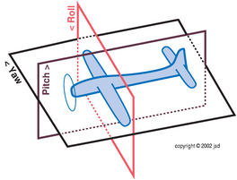
In aircraft (as well as boats and spacecraft) one way to describe rotations is in terms of yaw, pitch, and roll, as defined in figure 3. Rotations defined in this way require special treatment, because the axes are attached to the aircraft, not fixed in space. Therefore, if the aircraft turns, the new yaw-wise direction is different from the old yaw-wise direction ... and similarly for pitch and roll.
Using axes attached to the aircraft is entirely conventional and is entirely sensible from the pilot’s point of view.
It is remarkably easy to switch back and forth between axes attached to the aircraft and axes fixed in space, as we now explain:
Conventionally, the aircraft axes are called X, Y, and Z. That means yaw is a rotation in the XY plane, pitch is a rotation in the ZX plane, and roll is a rotation in the YZ plane.
Consider the following scenario: Initially, the aircraft axes {X, Y, Z} happen to coincide with the fixed-in-space axes {γ1, γ2, γ3}.
The pilot begins by performing some amount of roll. This is a rotation in the YZ plane, which is also a rotation in the γ2 γ3 plane. Let this rotation be represented by rotor r1. Next, the pilot performs some amount of pitch. This is a rotation in the ZX plane ... but it is not a rotation in the γ3 γ1 plane. We need to take into account that the current ZX plane is different from the original ZX plane. Let the second rotation be represented by the rotor r2 = a + b Z X, for suitable scalars a and b ... where Z and X are the current Z and X vectors.
It is easy to describe the current ZX plane in terms of things we already know. We can use the rotor r1 to rotate the original Z vector and also to rotate the original X vector. Specifically,
| (18) |
so the compound rotation r1 r2 can be expressed as
| (19) |
where it should be noted that on the LHS of the equation, r1 is the leftmost factor, while on the RHS of the equation, r1 is the rightmost factor. Also on the RHS, the factor in front of r1 is definitely not equal to r2, but looks hauntingly similar to r2, since it involves the same coefficients a and b, and involves vectors that were initially equal to Z and X.
This tells us something very interesting: If you know how to describe a rotation relative to the axes attached to the aircraft, you can also describe it relative to axes fixed in space using the same components, provided you multiply the rotors in the reverse order ... reversed relative to equation 5.
This trick about reversing the order of the operations is not dependent on Clifford algebra per se; it is a direct result of the basic geometry of rotations, and of how we have defined the XYZ axes. The basic logic is that when you apply the Nth rotation, if it comes to you described relative to the aircraft axes, you need to undo the previous N−1 rotations to understand how it looks relative to the original axes. You perform it, then re-do the other N−1 rotations. When you apply that logic at each step, the overall result is a complete end-for-end reversal of the order of the steps. You can find this discussed in classical mechanics books (e.g. Goldstein) under the heading of “passive versus active transformations”.
This trick is valuable because the same routines you use for keeping track of rotations relative to fixed axes can be used for keeping track of rotations relative to rotating axes, with essentially zero extra work. In fact it is so easy that people sometimes forget that the two schemes are conceptually different ... so be careful; remember which is which.
In section 4.2 and section 4.4 we used the notion that orthogonality corresponds to a 90 degree angle to construct some interesting rotors. In this section, we derive more general expressions, covering rotors with any angle whatsoever.
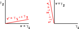
Let’s consider the situation shown on the left side of figure 4. We start with a vector v equal to γ1 and form another v′ by adding a tiny displacement vector in a perpendicular direction, so that:
| (20) |
Similar words apply to the right side of figure 4. We start with a vector v equal to γ2 and form another v′ by adding a tiny displacement vector in a perpendicular direction, so that:
| (21) |
Note that equation 20 has a plus sign, while equation 21 has a minus sign. This expresses a very important fact about the geometry of space. The minus sign occurs in the latter and not in the former because we are rotating in the γ1 γ2 direction, not in the opposite direction (γ2 γ1).
Rotating a sum of vectors is the same as rotating each summand separately, so we can combine equation 20 and equation 21 as follows:
| (22) |
We can take equation 22 as the definition of what we mean by rotation in the γ1 γ2 plane, in the limit of small angles. We shall soon verify that this definition is consistent with everything we already know about rotations. (Note that the angle є is measured in radians.)
We can use the vectors v and v′ from equation 20 to construct a rotor r, as follows:
| (23) |
where the last line is obtained simply by carrying out the indicated multiplications, and (as usual) simplifying by use of the normalization condition, equation 2. It is an easy exercise to show that taking the vectors v and v′ from equation 21 (instead of equation 20) would produce exactly the same rotor r in equation 23.
Let’s see what happens when we use this rotor to rotate something. We start with v = γ1 and create a new vector v″ as follows:
| (24) |
where the terms of order є2 can be neglected when є is small.
Then, comparing the last line of equation 24 with equation 20, we find that v″ is rotated relative to v by the angle 2є. That is, once again the rotation angle is twice the rotor angle.
Now we have all the fundamentals in place. We can start reaping the rewards.
The first thing to do is to consider larger rotations. Since we have constructed a rotationally-invariant representation of rotations, it is easy to represent repeated rotations, just by piling on additional copies of the rotation operator in accordance with equation 16.
Applying this idea, we can investigate what happens if we apply N copies of an infinitesimal rotation:
| v′ = (1 + є γ2 γ1)N v (1 + є γ1 γ2)N (25) |
where it is our intention that v′ be a vector rotated relative to v by the angle Nє.
Now, the powers on the RHS have a very interesting structure. In the limit of small є, we can write
| (1 + є γ1 γ2)N = exp(Nє γ1 γ2) (26) |
and we can expand the exponential in the familiar power series. (Equivalently, you can expand the LHS using the binomial theorem.) The result might look messy at first, but it can be greatly simplified by using the fact that γ1 γ2 γ1 γ2 = −1 whenever γ1 and γ2 are orthonormal and spacelike.
In the limit of large N, the first few terms of the series are, after simplification:
| exp(θ γ1 γ2) = 1 + θ γ1 γ2 − |
| − |
| θ3 γ1 γ2 + |
| + ⋯ (27) |
where any angle θ can be written as a multiple of є, that is, θ := Nє. Although є is small, we are not assuming that θ is small.
Collecting all the scalar terms, we recognize the series for cos(θ). The remaining terms remind us of the series for sin(θ). (Indeed, if you don’t recognize the power series for sin and cos functions, you could perfectly well use the power series to define those functions, and derive therefrom all the functions’ interesting properties, using the methods described in reference 9.)
In any case, we discover that:
| r(θ) = cos(θ) + γ1 γ2 sin(θ) (28) |
which is a wonderful result. We did not start out assuming that rotations would be periodic. All we did is turn the crank on the formalism, and it told us that rotations are periodic.
Let’s see what happens if we apply the rotor in equation 28 to a vector, according to the prescription in equation 5. We get
| (29) |
where we have used the trigonometric double-angle identities. We find that the rotor angle is half the rotation angle, even for non-infinitesimal angles.
By definition, spacetime refers to any system where we have one or more timelike dimensions, in addition to one or more spacelike dimensions. The most familiar example is D=1+3 spacetime, where we have one timelike dimension and three spacelike dimensions, but other possibilities should not be ruled out.
In spacetime, it is useful to categorize rotations as follows:
The physical interpretation is that boosting an object changes its velocity, just as rotating a line changes its slope. For more about the physical meaning of boosts, see reference 10.
The effect of a typical boost is depicted in figure 5. You can see that is analogous to – but not identical to – figure 4.
The geometry and trigonometry of boosts is very similar to the familiar geometry and trigonometry of spacelike rotations ... but not quite identical, as we now discuss.
Note: Some authors define “rotation” to include only spacelike rotations, excluding boosts. However, we wish to make a pedagogical and philosophical point, by treating the spacelike and timelike dimensions on the same footing. We shall see that they are as similar as they possibly could be, short of being absolutely identical. We should get used to living in a four-dimensional universe.
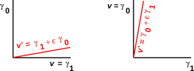
Let’s analyze a boost, following the same recipe as in section 4.
| (30) |
We can take equation 30 as the definition of what we mean by rotation in the γ0 γ1 plane, in the limit of small angles. This is analogous to – but not identical to – equation 22. In particular, the minus sign in equation 22 has been replaced by a plus sign in equation 30. This is the crucial difference between spacetime and ordinary Euclidean space.
Once again, we can construct rotors by forming the product of vectors:
| (31) |
where the last line was derived by multiplying the RHS by −1, and the ≅ sign should be interpreted as “having the same physical effect” since the rotor −r has the same physical effect as the rotor r, in accordance with equation 5.
Note that both of the factors (γ0) and (γ0 + є γ1) are timelike vectors. They come from the RHS of figure 5. Also: It is an easy exercise to show that the exact same value of r could have been obtained by multiplying two spacelike vectors from the LHS of figure 5, namely (γ1) and (γ1 + є γ0).
If we multiply together a large number of such rotors, we find an equation analogous to equation 27, except that all the minus signs are turned into plus signs, because γ0 γ1 γ0 γ1 = +1 for timelike γ0 and spacelike γ1. So instead of equation 28, we get
| r(θ) = cosh(θ) + γ1 γ0 sinh(θ) (32) |
that is, the rotor in the timelike direction is just the same, except that it uses hyperbolic trig functions where spacelike rotors use circular trig functions. In this equation θ is called the rotor angle.
The rotor in equation 32 can be written in various ways as the product of two unit vectors, either two spacelike unit vectors or two timelike unit vectors. Examples include:
| (33) |
If it’s not obvious, you should verify directly that the factor in square brackets is in fact a unit vector.
Let’s see what happens if we apply the rotor in equation 32 to a vector, according to the prescription in equation 5. In analogy to equation 29, we get
| (34) |
where the last line is exactly what we would expect to obtain as the result of boosting γ1 by a rapidity ρ. (See reference 11 for more about the idea of rapidity.) We see that the rapidity is twice the rotor angle, even for non-infinitesimal angles: ρ = 2θ. The calculation involves nothing more than carrying out the indicated multiplications, then using the hyperbolic trigonometric double-angle identities.
These are stunning results. They are simultaneously elegant, easy to use, and very powerful. See reference 10 for more about this.
Given two or more spacelike vectors {γ1, γ2, ⋯}, Clifford algebra gives us a nice representation of the rotation group. Given a timelike vector γ0 and the aforementioned spacelike vectors, we get a nice representation of the entire Lorentz group. That is, we can represent any combination of boosts and rotations in any direction ... and the formalism treats them all on the same footing, with a few caveats that will be discussed shortly.
We should have expected an intimate connection between boosts and rotations, because it has long been known that a sequence of boosts (not all in the same direction) can be used to produce a pure rotation.
Of course, space and spacetime have many things in common, but they are not exactly the same. First let’s consider what they have in common:
| In Euclidean space, γ1 is perpendicular to γ2. The product γ1 γ2 defines the plane of rotation, and plays a crucial role in the infinitesimal rotor r = 1 + є γ1 γ2. | In spacetime, γ0 is perpendicular to γ1. The product γ1 γ0 defines the plane of rotation, and plays a crucial role in the infinitesimal rotor r = 1 + є γ1 γ0. |
Specifically, if we recall the definition of r(θ)
from equation 28, γ1 γ2 is just the
derivative of r with respect to θ:
|
Specifically, if we recall the definition of r(θ)
from equation 32, γ1 γ0 is just the
derivative of r with respect to θ:
|
| The geometry of space can be quantified using circular trig functions, such as sin() and cos(). | The geometry of spacetime can be quantified using hyperbolic trig functions, such as sinh() and cosh(). |
Now let’s consider the ways in which space and spacetime differ:
| In the xy plane, you can turn x into y by a 90 degree rotation, and you can turn x into −x by a 180 degree rotation. | In the tx plane, you cannot turn t into x by any kind of rotation (including boosts) no matter how large or how small. Similarly you cannot turn t into −t (reversing the flow of time) by any kind of rotation. For more on this, see reference 10. |
| By itself, the product γ1 γ2 is a large-angle rotor. It is what we get from equation 28 when the rotor angle is π/2 radians. The scalar component of the rotor goes to zero at this point. | By itself, the product γ1 γ0 is not a rotor. It has gorm equal to −1, whereas all rotors must have gorm equal to +1. If you want a large boost involving γ1 γ0, you need to write something like √2 + γ1 γ0, which is what we get from equation 32 when the rotor angle is ln(1 + √2), i.e. about 0.881. The scalar component of the rotor never goes to zero. |
Let’s be clear: At some point you may be tempted to think of γ1 γ0 as a large angle boost, in analogy to γ1 γ2 ... but you must resist the temptation. That is, γ1 γ0 represents the plane of rotation, and it is the derivative of a rotor, but it is not a rotor unto itself. To understand why this must be so, consider the following argument: First of all, the set of all rotations is a continuous family of transformations; that is, for every possible rotation, there are other rotations nearby. The same goes for rotors: For every rotor, there are other rotors nearby. Secondly, a rotor with gorm equal to 1 cannot be near a rotor with gorm equal to -1. Thirdly, the rotor family is connected to the identity. That is, you can always set the rotor angle to zero in equation 32 and get a trivial rotor that represents the identity transformation. This trivial rotor has gorm equal to 1. All the rotors near the identity have gorm equal to 1, and by induction all the rotors in the world have gorm equal to 1.
Aficionados might wish to define the concept of improper rotor, namely elements of the even-grade subalgebra having gorm equal to −1. These represent improper rotations, including reflections and the like. Details are beyond the scope of the present discussion.
Also note that spacelike rotations and timelike rotations (aka boosts) do not cover all the possibilities. It is possible to have rotors such as q := 1 + θ γ2(γ0 + γ1) which is neither timelike nor spacelike. The trick is that γ0 + γ1 is a null vector. This q has gorm equal to 1 for all values of θ. This is not as weird as it might at first seem; such a rotor might describe a rocket that turns as it accelerates. This rotor q sits right on the dividing line, halfway between boosts and ordinary spacelike rotations. This is another reason why it is unhelpful to think of boosts as being different from rotations. It is better to lump them all together under the name “rotation”, no matter whether the plane of rotation is spacelike, timelike, or null. A boost in the x direction is just a rotation in the xt plane.
Also beware that when we draw a spacetime diagram, such as figure 5, we are using paper, which has two spacelike dimensions, to represent the γ0 γ1 plane, which in reality has one spacelike and one timelike dimension. As a result, the geometry of the diagram-on-paper is not an entirely faithful representation of the geometry of spacetime. In particular, the true notion of angle in the γ0 γ1 plane is not well represented in the diagram, especially when the angle is large. This makes it difficult to develop intuition about angles in spacetime. However, the mathematics is straightforward: just as the geometry of space can be quantified using circular trig functions, the geometry of spacetime can be quantified using hyperbolic trig functions, as you can see by comparing equation 29 with equation 34.
You might think that four dimensions is just like three dimensions, except 33% bigger. That is almost true, but not quite. There are some things that happen in four dimensions that are categorically different from what happens in three dimensions.
Unless otherwise stated, everything in this section applies to the case of four spacelike dimensions ... and also applies equally well to spacetime. That is, in this section we assume the fourth dimension is spacelike (γ4 γ4 = 1), but very similar remarks apply when it is timelike (γ4 γ4 = −1).
Executive summary: In this section, we will explain what we mean by the following:
- In any number of dimensions from two on up, any rotation (including boosts), and any combination of rotations (including boosts) can be represented by the equation V′ = r∼ V r where r is an element of the even-grade subalgebra.
- In two or three dimensions, but not four or more, we can represent an arbitrary rotor as the product of vectors.
That means that the mathematics always works. The mathematics gets more laborious as we move to higher dimensions, but the axioms remain the same, the logic remains the same, and the basic pattern of the calculations remains the same. You can use most of your intuition about two-dimensional and three-dimensional rotations as a guide to arbitrary rotations – including boosts – in four dimensions and higher.
One downside is that our ability to picture the most-general rotor as simply the product of two vectors is impaired in four dimensions and higher. Another downside is that four dimensions is considerably worse that 33% more laborious than three dimensions; it is typically about twice as laborious, as discussed in section 7.4.
Let’s do an example. Let’s pick two typical rotors (analogous to the ones we already encountered in equation 12) and see what happens when we multiply them. In four or more dimensions, the following example is reasonably typical:
| (37) |
We see that this product contains only even terms: a scalar term, a couple of bivector term, and a grade=4 term. (Some of these terms may vanish in special cases.)
If we are working in a three-dimensional space (which includes the case where we simply restrict our attention to a three-dimensional subset of a larger space), the situation is markedly simpler. There is no such thing as γ4 in three dimensions, so if we try to make something analogous to equation 37, the most complicated thing we can make is something like this:
| (38) |
where we have just replaced every occurrence of γ4 with γ2 and simplified the results using the axioms of Clifford algebra.
Equation 38 differs from equation 37 in two ways:
| In two or three dimensions, there cannot be any grade=4 term. If you try to construct a 4-blade of the form a∧b∧c∧d, the fourth factor (d) is necessarily linearly dependent on the previous factors, so the product necessarily vanishes. | In four or more dimensions, it is perfectly OK to have grade=4 terms. |
| In two or three dimensions, any object that is homogeneous of grade 2 is necessarily a 2-blade, i.e. the wedge product of two vectors. | In four or more dimensions, it is possible to have grade-2 objects that are not 2-blades, but rather the sum of 2-blades. |
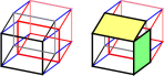
If you are good at visualizing things in four dimensions, figure 6 shows how to visualize a non-blade. On the left, just for reference, is a four-dimensional hypercube. On the right, we see two blades: one yellow, one green. These blades cannot be added edge-to-edge to form a single blade representing their sum, as we would do in three dimensions. We can’t do that, because the two blades have no edge in common. Indeed, no vector in the yellow plane is parallel to any vector in the green plane, and vice versa. Therefore the sum of these blades is homogeneous, but is not a blade.
There is a nice formalism for handling rotors in general (including both simple and non-simple rotors), as we now discuss: Start with all the elements in our Clifford algebra, and form a subset by throwing away any elements that contain any odd-grade terms, keeping only the even-grade blades and sums of even-grade blades. If you take any two elements from this subset and multiply them, you get another element of this subset. Therefore we say this subset is closed under multiplication. It is also true that this subset is closed under addition and subtraction. Therefore we conclude that this is not just a subset, it is a full-blown subalgebra, namely the even-grade subalgebra of our original Clifford algebra.
In all generality, we define a rotor to be an element of the even-grade subalgebra having gorm equal to 1. We define a simple rotor to be one containing no terms higher than grade=2. Some useful facts include:
When looking at equation 37, you may wonder how much trouble is caused by the fact that the grade=2 terms don’t form a blade. The answer is, surprisingly little trouble. It turns out that in equation 37, the overall rotor can be written as r = r1 r2. That is, r is not a simple rotor, but it can be visualized as the product of two simple rotors.
Note: in equation 37 the two rotors commute, i.e. r1 r2 = r2 r1. In four dimensions, an arbitrary rotor can always be represented as the product of two simple rotors that commute (hint: Gram-Schmidt orthogonalization), but this is not always the most natural representation; you are free to use two rotors that don’t commute, if you find that more convenient.
Also, if you are computing things in terms of components relative to some basis, as discussed in section 7.2, the same set of basis bivectors that is used to represent an arbitrary 2-blade is also sufficient to represent an arbitrary sum of 2-blades, so the existence of non-blades causes no extra work at all.
You should not imagine that there is a one-to-one relationship between rotors and rotations. Actually it is a two-to-one relationship. Any given rotation can be represented by two inequivalent rotors (r and −r). If you rotate something by 2π radians in any plane, you get back the same attitude, but the rotor picks up a minus sign. You need to rotate 4π radians to get back the original rotor.
This has practical significance if you have a computer program that needs to check whether a given attitude (represented by rotor r1) is close to the desired attitude (represented by rotor r2). It does not to suffice to see whether r1 is close to r2 in a component-by-component numerical sense; you have to check r1 against both r2 and −r2.
Before you decide that this is a defect in the Clifford algebra approach, note that there are situations in this world where a 4π rotation is equivalent to no rotation, but a 2π rotation is not. One example is the rotation of the wavefunction of a fermion. Examples can be found in the classical, macroscopic world: The Dirac string trick and the Philippine wine-glass trick. Details are beyond the scope of the present discussion.
The product-of-vectors representation may be even cleverer, even more profound than you initially thought.
In theoretical physics, almost anything worth saying can be said without reference to a particular basis.
However, when it comes time to do numerical calculations, it is often most practical to express vectors, bivectors, et cetera in terms of some chosen basis.
In a space where γ1, γ2, γ3 are the basis vectors, the natural basis for the bivectors is
| (39) |
That is, any plane can be represented as a linear combination of these three basis planes. (For more on this and its relationship to quaternions, see section 11.)
Using this basis for the bivectors we can represent any rotor in three dimensions by four numbers [x, y, z; w] where w is the scalar piece and x, y, and z are the coefficients that describe the bivector piece. Specifically,
| r = w + x ux + y uy + z uz (40) |
This expansion will be be put to good use in section 8.
Also: It is almost but not quite possible to represent a rotor in three dimensions using only three numbers, not four, because it is almost possible to infer the scalar piece using the normalization condition (equation 10). Even if you could infer the scalar piece, it would be more efficient to carry it around explicitly anyway, rather than recomputing it every time it was needed.
If you ever want to convert from the rotor representation to the matrix representation, here’s the procedure. Given a rotor of the form of the form w + x γ2γ3 + y γ3γ1 + z γ1γ2, the corresponding rotation matrix is
| ⎡ ⎢ ⎢ ⎣ |
| ⎤ ⎥ ⎥ ⎦ | (41) |
The Perl program mentioned in section 13 implements this matrix and uses it to convert rotors to matrices.
If you are wondering where equation 41 comes from, just apply the most-general rotor to the most-general vector, as follows:
| (w − x γ2γ3 − y γ3γ1 − z γ1γ2) [a γ1 + b γ2 + c γ3] (w + x γ2γ3 + y γ3γ1 + z γ1γ2) (42) |
Then just collect terms, as follows: How does the γ1 term depend on b? Those terms go in the middle of the top row of the matrix ... and similarly for all the other terms. In three (or fewer) dimensions, the trivector terms occur in pairs that cancel out, so they have no impact on the final result in equation 41.
We use the word clif to denote an arbitrary element of the Clifford algebra. A clif could be a vector, scalar, bivector, etc. – or a sum thereof. For more about the terminology, see reference 4.
The number of components required to describe a clif depends on the number of dimensions involved, i.e. the number of basis vectors in some chosen basis set. The first few cases are shown in this table, borrowed from reference 4:
| (43) |
where s means scalar, v means vector, b means bivector, t means trivector, and q means quadvector. You can see that it takes the form of Pascal’s triangle. On each row, the total number of components is 2D.
The even-grade components are shown in boldface. On each row, the number of even-grade components is 2(D−1)
For the purpose of representing rotors, you can ignore the odd-grade components in equation 43, but it is nice to have them there, because they help explain the number of even-grade components.
To make things really explicit, the number of components ordinarily required is as follows:
So we see that representing a rotor in four dimensions requires twice as many components as in three dimensions, which in turn requires twice as many components as in two dimensions.
In three-dimensional space, when you calculate the geometric product of two vectors, there will be four numbers you need to keep track of. This makes it significantly more compact than the rotation-matrix representation, which requires nine numbers in D=3.
In spacetime, a rotor can be specified using 8 numbers, which is significantly less than the matrix representation, which requires 16 numbers.
In D dimensions, a rotor is ordinarily represented using 2(D−1) numbers, while a matrix requires D2 numbers. The situation is summarized in the following table:
| Dimensionality | # of components | |
| rotor | matrix | |
| 3 | 4 | 9 |
| 4 | 8 | 16 |
| D | 2(D−1) | D2 |
We now move from the question of storage space to the question of computational effort required to calculate a compound rotation. If we use the rotor representation, all we need to do is multiply rotors, as suggested by equation 16. If we use the matrix representation, all we need to do is multiply matrices. The level of computational effort required is summarized in the following table:
| Dimensionality | multiplications required | |
| rotor | matrix | |
| 3 | 16 | 27 |
| 4 | 64 | 64 |
| D | 4(D−1) | D3 |
From this we can see that the rotor representation is computationally advantageous in D=3. The advantage vanishes in D=4, and turns into a disadvantage in very high-dimensional spaces.
Things get worse (but only slightly worse) when we ask how much computational effort is required to apply a given rotation to a vector. In the matrix representation, that involves just one matrix-vector product, while in the rotor representation, we need to perform two products, because there is a rotor on the left and on the right of the vector.
The situation is summarized in the following table:
| Dimensionality | multiplications required | |
| rotor | matrix | |
| 3 | 28 | 9 |
| 4 | 96 | 16 |
| D | 4(D−1) + O(D*2(D−1)) | D2 |
This is unflattering to the rotor representation ... but we should keep things in perspective, as we now discuss:
To summarize the overall situation:
Here is a very practical example. In VRML (virtual reality modeling language) a rotation is represented by specifying the axis of rotation and the amount of rotation. Specifically, the amount of rotation is specified in radians, and the axis must be specified as a unit vector. (If you inadvertently use a non-unit vector, weird things will happen.) For example, a 90 degree rotation around the X axis is represented by (1 0 0 1.5708).
It is easy to convert back and forth between this representation and the geometric-algebra representation. If the VRML representation is (X, Y, Z, θ), the scalar piece of the rotor is cos(θ/2) and the components of the bivector piece are [X sin(θ/2), Y sin(θ/2), Z sin(θ/2)].
If you want to calculate a compound rotation, the easiest method is to convert to the rotor representation, multiply the rotors, and then convert back to the VRML representation. This approach has several advantages, including:
The perl program mentioned in Reference 8 knows how to perform this calculation. The principle of operation of the program is as follows: Let the first VRML rotation be (X1, Y1, Z1, θ1). Then the corresponding rotor is
| (44) |
where ux etc. are defined by equation 39.
We define the second rotor r2 in the corresponding way, i.e. just change “1” to “2” everywhere in equation 44.
To calculate the compound rotation, we just multiply the rotors. Each rotor is represented by four numbers, so (before simplification) there will be sixteen terms in the product, namely:
| (45) |
and then it’s just a matter of simplifying by collecting like terms. The result is a rotor, represented by four numbers in the usual way.
Here is an amusing tangential thought: The program takes the arccosine at one point. I have learned through bitter experience to be careful with arccosines. The problem is that when the input routine takes the cosine of θ, it is insensitive to the sign of θ. That is, cos(θ) looks a whole lot like cos(−θ). Then when the output routine takes the arccosine, you might or might not get back the original θ, depending on whether or not it was in the top half or the bottom half of the unit circle. The only reason this is not a problem for the code in reference 8 is that the input routine also calculates sin(θ) and factors it into the bivector piece of the rotor. So if your rotation angle is in the bottom half of the unit circle, it will get flipped to the top half, but this is OK because the axis of rotation will get flipped end-for-end.
The reflection of a vector v in a flat mirror can be expressed by the simple formula:
| (46) |
where a is a unit vector in the direction normal to the mirror. Obviously you can use −a instead of a and it doesn’t change anything.
Here are some examples:
| (47) |
In three-dimensional space, a normal in the x direction corresponds to a mirror in the yz plane. In four-dimensional spacetime, a normal in the x direction corresponds to a mirror in the xzt hyperplane, which makes sense if you think of it as the world-line of a stationary mirror.
World-lines cannot be spacelike, so you cannot have a mirror in the xyz hyperplane, and the normal cannot be timelike. However, a mirror that is in motion can have a smallish timelike component to its normal. Therefore it is worthwhile to extend the previous equation. As is so often the case, the timelike component behaves “almost” but not quite the same as the other components.
| (48) |
For example, let’s consider a mirror perpendicular to the x axis. In three-dimensional space, the mirror resides in the yz plane. In spacetime, if the mirror is stationary, the world-line of the mirror resides in the yzt hyperplane. In either case, the unit normal vector is x, as you can verify by direct computation.
Hint: A vector is perpendicular to a plane if and only if it is perpendicular to every vector in the plane. This reduces the workload when checking to see whether things are perpendicular. Further hint: by definition, two vectors are perpendicular if their dot product is zero. In the present example, x is obviously perpendicular to y, z, and t.
Suppose there is an incoming photon, with 4-momentum p1=[1,−1,0,0]. That corresponds to normal incidence. After it reflects off the mirror, the momentum will be:
| (49) |
which makes sense. The 3-velocity of the photon has been reversed.
Now let’s set the mirror in motion in the x direction. The moving mirror resides in the yz(ct+sx) hyperplane, where c=cosh(ρ), s=sinh(ρ), and ρ is the rapidity. The expression for the hyperplane comes from boosting each of the constituent vectors in the obvious way. The unit normal is not x but rather cx+st. Again it is straightforward to verify that this is perpendicular to the hyperplane.
Using the same incident photon, namely p1=[1,−1,0,0], the reflection from the moving mirror will be
| (50) |
That’s exactly what you would get by reversing the direction of motion of the photon, and then boosting it by twice the rapidity of the mirror. This factor of 2 should be familiar from the ordinary non-relativistic mechanics of a batted ball: you need to boost once to get the ball into the rest frame of the bat, then perform a simple reflection against the stationary bat, and the boost again to get the result into the lab frame.
Let’s move on to a more complicated but more interesting example: Consider a mirror at 45∘ to the x and y axes. In three-dimensional space we consider it to reside in the √½(x−y)z plane. In spacetime, if the mirror is stationary, its world-line resides in the √½(x−y)zt hyperplane. In either case, the unit normal is √½(x+y), as you can verify by direct computation.
Now let’s set the mirror in motion in the x direction. The moving mirror resides in the √½(cx+st−y)z(ct+sx) hyperplane. The unit normal is √½(cx+st+y). Again it is straightforward to verify that this vector is perpendicular to the mirror.
I leave it as an exercise for the reader to work out what happens to p1 when it reflects off this mirror. This is the non-stationary, non-normal-incidence case.
It is not super-important to the current discussion, but there is a deep connection between rotations and reflections. If you want details, see reference 7, but we include a brief overview here.
In general, if you apply the same reflection operator twice, you get back where you started. Reflecting in one mirror then reflecting again in a different mirror undoes most of the effects of the reflection – in particular it undoes the inversion – but it produces a rotation. The amount of rotation is twice the angle between the two mirrors.
This means that given two vectors that span a half-angle, we can use them to represent a rotation through the full angle as follows: First, reflect everything in the mirror perpendicular to the first vector, then reflect everything again in the mirror perpendicular to the second vector. This is entirely equivalent to the procedure described in section 4; it is just another way of looking at things.
In D=2, the mirror is the D−1 = 1 dimensional line perpendicular to the given vector. In D=3, the mirror is the D−1 = 2 dimensional plane perpendicular to the given vector. In D=4, the mirror is the D−1 = 3 dimensional hyperplane perpendicular to the given vector.
This interpretation in terms of reflections makes it pretty obvious that this representation is Lorentz-invariant.
Remember that the rotor angle is half the rotation angle. This can be a source of confusion if you’re not careful.
In section 9.3, section 2.1, and section 4.1, we considered two vectors that spanned half the angle of the desired rotation. We now consider the case where there are two vectors that span the full angle. This is not recommended. In particular, it is ambiguous when the two vectors are oppositely directed.
Here’s the general procedure. If you want the rotation that turns P to the direction of Q, construct the normalized versions Pnorm and Qnorm. Then calculate the bisector B := Pnorm + Qnorm)/2. In the special case when the bisector is zero, rotate 180∘ in some arbitrarily-chosen plane containing P. Otherwise, calculate the geometric product PB, and then normalize it.
There is a one-to-one correspondence between quaternions and a subalgebra of Clifford algebra, namely the subalgebra containing only scalars and bivectors.
The basis bivectors in equation 39 are identical to the I, J, K basis quaternions, except each is missing a minus sign. Specifically, we define the quaternions I, J, and K according to:
| (51) |
The fourth basis quaternion is the plain old scalar 1.
By direct application of the Clifford Algebra axioms (equation 1 and equation 2), you can verify Hamilton’s celebrated identities I2 = J2 = K2 = IJK = −1 (reference 1).
The advantage of the Clifford Algebra approach is that you don’t need to spend any effort learning the algebra of quaternions. Once you know the axioms of Clifford Algebra, you get quaternions (and a lot of other things) for free.
(The quaternions we have called I, J, and K are more conventionally written as lower-case i, j, and k, but in this document we capitalize them, for reasons that will become obvious in a moment.)
Another set of objects that serve as generators of rotations are the Pauli spin matrices, namely:
| (52) |
These behave like the I, J, K quaternions, except each is missing a factor of i, where i := √(−1). Specifically, you can verify that if we redefine I:=iσx, J:=iσy, and J:=iσz then once again we can write Hamilton’s identities, namely I2 = J2 = K2 = IJK = −1.
The three Pauli matrices of course go along with a fourth matrix, the unit matrix:
| (53) |
Note: In this section, all rotations live in D=3 space, unless otherwise specified.
Let’s imagine you are playing charades, and you want to portray a rotation, a very specific rotation. There are various approaches you could take:
You can make this seem more scientific by choosing the “object” to be a triad of linearly-independent vectors. You need to label the vectors, so you can keep track of which is which. Then the length of the vectors doesn’t matter, so we can WLoG3 take them to be unit vectors. As before, you need to depict the triad twice, once before and once after rotation.
The formal mathematical version of this approach consists of writing down the rotation matrix. The left column of the matrix shows where the X unit vector winds up after rotation; the middle column shows where the Y unit vector winds up, and the right column shows where the Z unit vector winds up.
Using a matrix to rotate a vector is computationally efficient, as discussed in section 7.4.
The downside is that it is inconvenient to convert from the matrix representation to other representations.
If you are doing a lot of calculations, you can keep the basis constant, so the three Euler angles are the only variables. This means you only need to carry around three variables, which would seem to be an improvement over the rotation-matrix representation, which requires carrying around nine variables.
Euler angles are semi-reasonable for some applications, especially if the pitch angle and the bank angle4 always remain small, as they do in ordinary non-aerobatic flying. But there are many drawbacks. For one thing, there are nasty singularities, such as the following: suppose you pitch up 89 degrees. Your heading5 is unchanged, and your bank angle is unchanged. So far so good ... but now continue the pitch-wise motion another two degrees. Your heading is now reversed (180 degrees from where you were a moment ago) and your bank angle is upside down (also 180 degrees from where it was a moment ago).
Any scheme for representing rotations (in D=3 space) using only three variables will have singularities. There’s no way around it.
Even if you stay away from the singularities, if you want to describe the results of two consecutive rotations, the mathematics of Euler angles is not very pretty.
Because the Euler angles depend on a particular choice of basis, they represent rotations in a way that is not rotation-invariant ... which is pathetic. Of course they have no chance of being relativistically invariant.
This can be formalized in terms of the so-called Rodrigues vector. The direction of the Rodrigues vector indicates the axis of rotation, and the length represents the amount of rotation.
This representation is not as elegant or as useful as one might have hoped. In particular, if you compound two rotations, the result is not represented by the sum of the Rodrigues vectors (nor the product, nor any other simple vector operation).
The Rodrigues vector is not relativistically invariant.
Also, this approach is restricted to D=3 space only. In D=2 flatland, it is not necessary – nor even possible – to specify the direction of rotation as a vector. In D=4 or higher, including D=1+3 spacetime, it is again impossible to represent the direction of rotation as a vector. In D=4, it takes 6 numbers to specify the direction of rotation, but a 4-vector has only 4 components. The way out of this difficulty can be found in the following item.
This can be formalized as the product of two vectors in the plane, as discussed in section 2.
Note: For all the representations discussed here, we have represented only the amount of rotation and the orientation of the plane of rotation; we have not attempted to represent the location of the center of the rotation.
However, there is a theorem that says that a rotation about one center can be decomposed into a rotation around another center, plus a pure translation. We assume everybody understands how to represent translations. So for simplicity, we consider only rotations around the origin.
I wrote a “Clifford algebra desk calculator” program. It knows how to do addition, subtraction, dot product, wedge product, full geometric product, reverse, hodge dual, and so forth. Most of the features work in arbitrarily many dimensions.
Here is the program’s help message. See also reference 8.
Desk calculator for Clifford algebra in arbitrarily many
Euclidean dimensions.  (No Minkowski space yet; sorry.)

Usage:  ./cliffer [options]

Command-line options include
  -h      print this message (and exit immediately).
  -v      increase verbosity.
  -i fn   take input from file 'fn'.
  -pre fn take preliminary input from file 'fn'.
  --      take input from STDIN

If no input files are specified with -i or --, the default is an
implicit '--'.  Note that -i and -pre can be used multiple times.
All -pre files are processed before any -i files.

      Advanced usage: If you want to make an input file into a
      self-executing script, you can use "#! /path/to/cliffer -i" as
      the first line.  Similarly, if you want to do some
      initialization and then read from standard input, you can use
      "#! /path/to/cliffer -pre" as the first line.

Ordinary usage example:
  # compound rotation:  two 90 degree rotations
  # makes a 120 degree rotation about the 1,1,1 diagonal:
  echo -e "1 0 0 90° vrml 0 0 1 90° vrml mul @v" | cliffer
Result:
          0.57735 0.57735 0.57735 2.09440 = 120.0000°

Explanation:
  *) Push a rotation operator onto the stack, by
  giving four numbers in VRML format
     X Y Z theta
  followed by the "vrml" keyword.
  *) Push another rotation operator onto the stack,
  in the same way.
  *) Multiply them together using the "mul" keyword.
  *) Pop the result and print it in VRML format using
    the "@v" keyword

On input, we expect all angles to be in radians.  You can convert
  from degrees to radians using the "deg" operator, which can be
  abbreviated to "°" (the degree symbol).  Hint: Alt-0 on some
  keyboards.
  As a special case, on input, a number with suffix "d" (with no
  spaces between the number and the "d") is converted from degrees to
  radians.
    echo "90° sin @" | cliffer
    echo "90 ° sin @" | cliffer
    echo "90d sin @" | cliffer
  are each equivalent to
    echo "pi 2 div sin @" | cliffer

Input words can be spread across as many lines (or as few) as you
  wish.  If input is from an interactive terminal, any error causes
  the rest of the current line to be thrown away, but the program does
  not exit.  In the non-interactive case, any error causes the program
  to exit.

On input, a comma or tab is equivalent to a space.  Multiple spaces
are equivalent to a single space.

Note on VRML format:  X Y Z theta
  [X Y Z] is a vector specifying the axis of rotation,
  and theta specifies the amount of rotation around that axis.
  VRML requires [X Y Z] to be normalized as a unit vector,
  but we are more tolerant;  we will normalize it for you.
  VRML requires theta to be measured in radians.

Also note that on input, the VRML operator accepts either four
  numbers, or one 3-component vector plus one scalar, as in the
  following example.

Same as previous example, with more output:
  echo -e "[1 0 0] 90° vrml dup @v dup @m
           [0 0 1] -90° vrml rev mul dup @v @m" | cliffer
Result:
        1.00000 0.00000 0.00000 1.57080 =  90.0000°
           [  1.00000  0.00000  0.00000 ]
           [  0.00000  0.00000 -1.00000 ]
           [  0.00000  1.00000  0.00000 ]
        0.57735 0.57735 0.57735 2.09440 = 120.0000°
           [  0.00000  0.00000  1.00000 ]
           [  1.00000  0.00000  0.00000 ]
           [  0.00000  1.00000  0.00000 ]

Even fancier:  Multiply two vectors to create a bivector,
then use that to crank a vector:
  echo -e "[ 1 0 0 ] [ 1 1 0 ] mul normalize [ 0 1 0 ] crank @" \
   | ./cliffer
Result:
    [-1, 0, 0]

Another example:  Calculate the angle between two vectors:
  echo -e "[ -1 0 0 ] [ 1 1 0 ] mul normalize rangle @a" | ./cliffer
Result:
    2.35619 = 135.0000°

Example: Powers: Exponentiate a quaternion.  Find rotor that rotates
only half as much:
   echo -e "[ 1 0 0 ] [ 0 1 0 ] mul 2 mul dup rangle @a " \
        " .5 pow dup rangle @a @" | ./cliffer
Result:
    1.57080 =  90.0000°
    0.78540 =  45.0000°
    1 + [0, 0, 1]§

Example:  Take the 4th root using pow, then take the fourth
power using direct multiplication of quaternions:
  echo "[ 1 0 0 ] [ 0 1 0 ] mul dup @v
  .25 pow dup @v dup mul dup mul @v" | ./cliffer
Result
    0.00000 0.00000 1.00000 3.14159 = 180.0000°
    0.00000 0.00000 1.00000 0.78540 =  45.0000°
    0.00000 0.00000 1.00000 3.14159 = 180.0000°

More systematic testing:
   ./cliffer.test1

The following operators have been implemented:
help    help message
listops list all operators
=== Unary operators
pop     remove top item from stack
neg     negate: multiply by -1
deg     convert number from radians to degrees
dup     duplicate top item on stack
gorm    gorm i.e. scalar part of V~ V
norm    norm i.e. sqrt(gorm}
normalize divide top item by its norm
rev     clifford '~' operator, reverse basis vectors
hodge   hodge dual aka unary '§' operator; alt-' on some keyboards
gradesel given C and s, find the grade-s part of C
rangle  calculate rotor angle
=== Binary operators
exch    exchange top two items on stack
codot   multiply corresponding components, then sum
add     add top two items on stack
sub     sub top two items on stack
mul     multiply top two items on stack (in subspace if possible)
cmul    promote A and B to clifs, then multiply them
div     divide clif A by scalar B
dot     promote A and B to clifs, then take dot product
wedge   promote A and B to clifs, then take wedge product
cross   the hodge of the wedge (familiar as cross product in 3D)
crank   calculate R~ V R
pow     calculate Nth power of scalar or quat
sqrt    calculate square root of power of scalar or quat
=== Constructors
[       mark the beginning of a vector
]       construct vector by popping to mark
unpack  unpack a vector, quat, or clif; push its contents (normal order)
dimset  project object onto N-dimensional Clifford algebra
unbave  top unit basis vector in N dimensions
ups     unit pseudo-scalar in N dimensions
pi      push pi onto the stack
vrml    construct a quaternion from VRML representation x,y,z,theta
clif    take a vector in D=2**n, construct a clif in D=n
	Note:  You can do the opposite via '[ exch unpack ]'
=== Printout operators
setbasis set basis mode, 0=abcdef 1=xyzabc
dump    show everything on stack, leave it unchanged
@       compactly show item of any type, D=3 (then remove it)
@m      show quaternion, formatted as a rotation matrix (then remove it)
@v      show quaternion, formatted in VRML style (then remove it)
@a      show angle, formatted in radian and degrees (then remove it)
@x      print clif of any grade, row by row
=== Math library functions:
       sin    cos    tan    sec    csc    cot
       sinh   cosh   tanh   asin   acos   atan
       asinh  acosh  atanh  ln     log2   log10
       exp    atan2
|