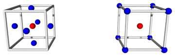
Figure 1: 2N+1 versus 2N+1
Loosely speaking, given a formula and some input variables with error bars, we wish to calculate the output variable and its error bars. To say the same thing more carefully: We know the distribution over input values, and we wish to calculate the distribution over output values.
• This documentation links to several live examples using the Uncertainty Calculator. For these to work, your browser must allow a popup window. • In any case, you are always free to start a standalone (non-popup) copy of the Uncertainty Calculator
• This is the simple version. There is also a much fancier version, with graphics and Monte Carlo.
Fill in nominal values and error bars for the input variables you plan to use: x, y, and z. Also enter a mathematical formula that maps the input variables to the desired output. Then press <Enter> in any of the input boxes, or click the Go button.
Let’s start with something ultra-simple, namely the example. In this case there are no variables. The formula is just the number 13. The calculated result is 13 with no uncertainty.
Here’s another example, almost as simple, namely the example. The formula is simply “x”, which means the output is the same as the x-input. The x-input is drawn from a distribution that is rectangular, is centered at 10, and has a half-width at half-maximum (HWHM) of 3. The calculated result is the same.
The general rule is this: When we write A±B, we are describing a distribution, where A specifies the nominal value of the distribution, while B specifies the error bars.
This is the Crank Three Times method. There is nothing tricky or complicated about it. The same result could be obtained using a pocket calculator. (The Uncertainty Calculator has additional features, but we don’t need them for present purposes.)
You can specify the error bar as a plain old number, or in terms of percentage, or in terms of ppm (parts per million), as demonstrated in the example. The two input distributions have exactly the same uncertainty, although it is specified in dissimilar ways.
You can also change the names of the variables, as shown in the example. The slickest way to change the name of the result variable is to write an assignment statement in last step in the formula, as demonstrated in the aforementioned example. The advantage is that the new name does not take effect until after the formula has been evaluated. In contrast, input variables must be renamed by hand.
Suppose there are N input variables, drawn from independent random distributions. In 2N+1 mode, also known as axis mode, the calculator checks all 2N faces of the hypercube, specifically the centers of the faces, allowing only one variable to fluctuate at a time. The +1 comes from the point at the center of the hypercube. If you have a huge number of fluctuating variables, this mode leads to an underestimate of the RMS error, since in reality two or more variables can fluctuate at the same time.
In contrast, in 2N+1 mode, also known as corner mode, then the calculator checks all 2N corners of the hypercube, looking for the worst-case combination of 1-bar-length fluctuations. Once again, the +1 comes from the point at the center of the hypercube. If you have a huge number of variables, this mode leads to a calculated error bar on the distribution over results that is an overestimate of the RMS error.
The Uncertainty Calculator always carries out both modes of calculation; the button near the top right corner merely selects which of the two results is displayed.
In particular, consider the case where we have two input variables, x and y, each drawn from a rectangular distribution, i.e. uniform over some interval. Then the worst-case error bar (half-width at baseline) is the same as the HWHM (half-width at half maximum). Then the distribution over the sum (x+y) is a trapezoid, with the following properties:
Beware that if you have a huge number of variables, computing the worst-case error bar is usually not what you want, because the worst case will be exponentially unlikely.
If the two input distributions are Gaussian (not rectangular), then axis mode will underestimate the uncertainty on the distribution over x+y, while corner mode will overestimate it. This can be understood in more detail by plotting the Monte Carlo data.
The input distributions x, y, and z are independent. The calculator constructs them to be so. You must structure your calculation accordingly. That is, if some preliminary formulation of the calculation uses distributions that are correlated, you need to reformulate it in terms of distributions that aren’t. The example provides a fine example of this. The most obvious preliminary formulation uses the three abundance percentages directly. However, they highly correlated, because they are constrained to add up to 100%. So we reformulate the calculation in terms of two uncorrelated distributions, x and y, which we use to model the two experimentally-determined ratios. For the next level of detail, see reference 1. The two-distribution approach is less obvious but more natural, i.e. closer to the actual physics.
The inputs can be considered “Step 0” of the calculation. At every step after that, Crank Three Times will automatically take care of correlations that arise in the course of the calculation, as they so often do.
We emphasize that the variable x is just a number, i.e. a zero-sized pointlike point, with no uncertainty and no error bars whatsoever. In our notation, {x} refers to a set of x-values. Similarly, A±B refers to a distribution, which is mostly just a of points. The distribution usually has some width, whereas an individual data point never does. The width essentially defines what is meant by uncertainty. A point is different from a distribution, as surely as a scalar is different from an infinite-dimensional vector.
In particular: Even though the Uncertainty Calculator is sometimes mentioned in the same sentence as “uncertainty propagation software” or “error propagation software”, it does not propagate the uncertainty per se through the calculation. It calculates the uncertainty, but only at the end, and not via step-by-step propagation. The only things that get propagated are zero-sized pointlike points. In a multi-step calculation, the intermediate steps do not have – or need – any way of representing uncertainty. The intermediate steps do not have – or need – error bars or significant figures or anything like that. This is important for multiple reasons:
If the calculated result-distribution has lopsided error bars, the Uncertainty Calculator will show the upper and lower error bars separately. This is a warning. It means there is something fishy with the model you are using. In contrast, other methods such as «sig figs» and/or «propagation of error bars» will give you wrong answers without warning.
Lopsided error bars mean you have reached the limit of what you can safely do using only Crank Three Times. To figure out what’s going on, you need more powerful tools, such as the Monte Carlo features provided by the fancy version of the Uncertainty Calculator.
In all cases our results are shown using enough digits so that the roundoff error is at most 1/20th of an error bar.
This requires one or two digits more than would be permitted by «sig figs». That’s because we want to get the right answer, without excessive roundoff error. «Sig figs» tries to use one numeral to represent two numbers, namely the nominal value and the uncertainty, which is a terrible idea. Use the A±B representation instead. Furthermore, «sig figs» requires excessive rounding, which is incompatible with getting the right answer.
Just because you can calculate the uncertainty, it doesn’t necessarily mean you should. It doesn’t guarantee that the result means anything. In the real world, sometimes the uncertainty of a result is determined by the uncertainty of the inputs you plug into the calculation – but sometimes it isn’t, due to unobserved variables and/or built-in biases in the model.
On the Uncertainty Calculator interface, click on the red-and-black
wheel symbol
![]() to turn off
the to reveal the Monte Carlo features. There is separate
documentation for the
fancy version.
to turn off
the to reveal the Monte Carlo features. There is separate
documentation for the
fancy version.