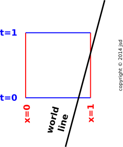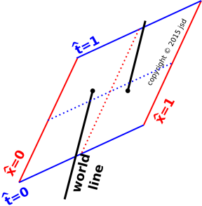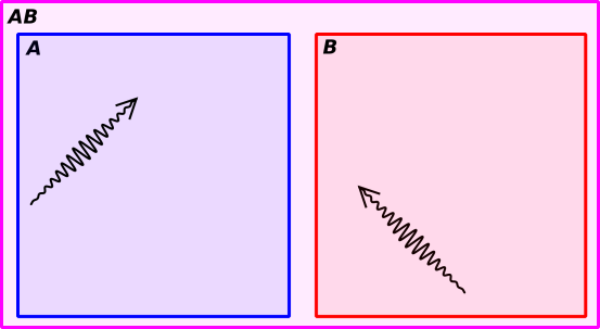
Figure 1: World-line of Stationary Parcel
When electric charge flows from place to place, it obeys a local conservation law. By that we mean something very specific:
Any decrease in the amount of charge in a given region of space
must be exactly balanced by
a simultaneous increase in the amount of charge in an adjacent region of space.
We can express the same idea in the form of an equation:
| (1) |
The word “flow” in this expression has a very precise technical meaning, closely corresponding to one of the meanings it has in everyday life. Specifically: Charge cannot be created or destroyed, but it can flow one from one region to another. Any decrease in one region is exactly balanced by a simultaneous increase in an adjacent region.
(By way of contrast, if you want an example of something that flows but is not conserved, consider “the flow of ideas”. You can give me an idea without decreasing your own stock of ideas. As usual, flow refers to spreading from one region to a neighboring region.)
At this point we have three ideas on the table: conservation, change, and flow. In accordance with equation 1, we can understand conservation as a combination of change plus just the right amount of flow.
To repeat: electric charge cannot change arbitrarily; only certain types of changes are allowed. The relationship between the broad concept of “change” and the more-precise concept of “conservation” can be summarized as follows:
| (2) |
The use of the world “simultaneity” causes some people to wonder
whether equation 2 can be relativistically correct. Well, it
turns out that this equation is 100% kosher, relativistically and
otherwise. We get into trouble with relativity when we talk about
simultaneity at a distance, but since we are taking about
adjacent changes – zero distance – there is no problem with
simultaneity. Indeed, our notion of conservation is beautifully
matched to modern notions of relativity. In spacetime, local
conservation can be expressed in elegant, informative, and
easy-to-visualize form, in terms of the continuity of world
lines. This is discussed in section 2.
To be useful – or even correct – the conservation law must be local, as discussed in section 2.3. It must apply to every region in spacetime, including small open regions where the charge is not constant. Charge is always conserved, even though it is not always constant, as discussed in section 2.4.
As a corollary, as a special case of equation 2:
This stands in contrast to the general case, where conservation does not imply constancy, nor vice versa. This is discussed in section 2.4.
To summarize: The laws of physics do not permit charge to disappear now and reappear later. Similarly the laws do not permit charge to disappear from here and reappear at some distant place.
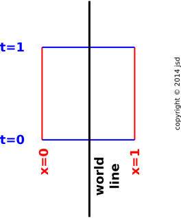
An ordinary box in D=3 space has six faces. We can call them the ± x faces, the ± y faces, and the ± z faces. In D=4 spacetime, the corresponding object has eight faces, namely two ± t faces in addition to the six spatial faces.
Now let’s draw some spacetime diagrams. For simplicity we will conceal the y and z dimensions, and portray only the ± t and ± x faces of the box.
Figure 1 shows the world-line of a stationary parcel of electrical charge sitting at the location of our box. The world-line enters on the t=0 face and exits on the t=1 face. In other words, it was initially within the spatial extent of our box, and it remained so.
World-lines crossing the ± t faces contribute to the time derivative of the amount of charge in the box. In figure 1, there are two equal and opposite contributions, namely one flowing in at t=0, and one flowing out at t=1.
| In 4-dimensional spacetime terms: The charge is flowing in the time direction only. | In 3-dimensional spatial terms: The charge is not flowing at all. It just sits there. The amount of charge within the spatial extent of the box is the same at t=0 and t=1, so the amount of charge in that spatial region is constant, i.e. not changing with time. |
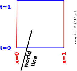
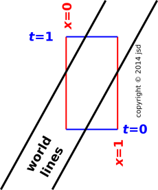
We now consider what happens when the charge is non-stationary, as shown in figure 2. The world-line enters via the t=0 face and exits via the x=1 face. In other words, the parcel was initially within the spatial extent of our box, but then it departed toward the right.
In this case, the amount of charge in the spatial box at t=1 is less than the amount of charge at t=0. The charge is not locally constant, but it is locally conserved. The charge wasn’t destroyed, it just flowed across the x=1 boundary into the neighboring region.
We will make this more quantitative in a moment. To make this useful, we will need to quantify the net flow across the ± x boundaries. It helps to know something about velocity and charge density.
You can see where this line of reasoning is leading. The following notions are formally equivalent:
We now consider a non-conserved object, such as a muon. Here is the world-line of a muon that decays within the box; the world line enters the box but doesn’t go out again:
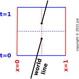
Here are some trickier examples of non-conservation. In figure 4, the particle disappears and then reappears at a later time. Electric charge does not behave like this. The law of conservation of charge forbids it. In particular, if we divide the region into an early half and a late half, we now have two regions, both of which exhibit gross non-conservation. The lesson here is that the conservation is not equivalent to saying that you end up with the same amount you started with. The conservation law applies not just at the starting time and ending time, but at every time along the way.
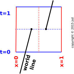
Similarly, in figure 5, the particle disappears at one location and reappears at some other location. Electric charge does not behave like this. The law of conservation of charge forbids it. In particular, if we divide the region into left half and a right half, we now have two regions, both of which exhibit gross non-conservation. The lesson here is that the conservation is not equivalent to saying that the total amount is constant over time. The conservation law applies not just to the universe as a whole, but also to every region and subregion.
It must be emphasized that conservation of charge is a local conservation law. The property of “locality” is crucial, for at least two reasons, as we shall see.
It is possible to have global conservation without local conservation, as shown in figure 5. If we consider only the large region from x=0 to x=1, there is no change in the charge inside, and no flow across the ±x boundaries, so we have conservation in accordance with equation 1.
The first huge problem with global conservation is that it is not useful in practice. If some charge disappears from your laboratory and reappears somewhere far, far away, you have no way of knowing whether it is really conserved. You have no way of checking. An unenforceable law is useless.
The second huge problem manifests itself when we consider a second reference frame, moving relative to the first, in accordance with the laws of special relativity. The situation is shown in figure 7. In this figure, the world lines are exactly the same as in figure 6 (and also figure 5); only the reference frame is changed. Whereas an ordinary rotation in the xy plane rotates the x and y contour lines the same way, a spacetime rotation in the xt plane tilts the x contours one way and the t contours the other way. For details, see reference 1. In figure 7, the amount of tilt corresponds to a x^t^ frame that is moving at half the speed of light (relative to the xt frame).
The point of all this is that in the x^t^ frame, the particle disappears later than time t^=0.5 and reappears earlier than that. Therefore even though the amount of charge is globally constant relative to the xt frame, it is not constant relative to the x^t^ frame. Since the laws of physics are required to work in any reference frame, we see that any notion of non-local conservation is dead on arrival. In the real world, i.e. in spacetime, non-local conservation is almost no conservation at all.1
It is important to distinguish the notion of constancy from the notion of conservation:
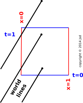
Imagine a fluid that has the same velocity and the same charge-density everywhere. An example of such a situation is shown in figure 8.
In this case, the amount of charge in the box is constant, because whenever a parcel of charge leaves via the x=0 face, an equivalent amount of charge is entering via the x=1 face. Contrast this with figure 2, where the charge flowed out and was not replaced. This non-replacement could occur because the charge density was lower off to the left, and/or the velocity was lower off to the left. So we see we need to be concerned with
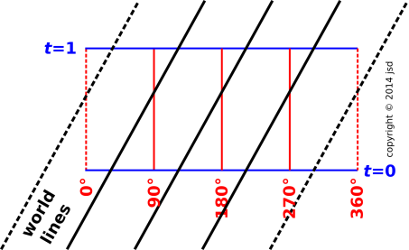
A particularly interesting case of constancy with flow and replacement is steady flow around a loop, as shown in figure 9. The diagram is subject to periodic boundary conditions. That is, the two dashed worldlines are the same worldline. Also the two dashed red boundaries are the same boundary. Every time a particle flows out of one compartment it is replaced by another particle flowing in.
We have just seen constancy with conservation, via outflow compensated by inflow. We now constrast that against constancy without conservation, via annihilation and inflow. This shown in figure 10. You can see that the number of objects in the region of interest is constant, because every time one of them is destroyed it is replaced.
A real-life example of this concerns the number of working light-bulbs in a room. The number of working light bulbs is not a conserved quantity, but the number is approximately constant, because every time a light bulb is destroyed you replace it.
Another example along the same lines is a continuous-flow reactor in a chemical plant, where chemicals of type A flow in and chemicals of type B flow out.
To be explicit: Conservation does not imply constancy, nor vice versa. Change does not imply non-conservation, nor vice versa. All four of the possibilities have already been illustrated:
| constant | non-constant | ||||
| conservation | Figure 1 (static) | Figure 2 (outflow) | |||
| Figure 8 (steady flow) | |||||
| non-conservation | Figure 10 (steady replacement) | Figure 3 (annihilation) |
As touched upon section 1, if you integrate the local conservation law over all space, you can derive a global conservation law as a corollary. It is true that global conservation is the same as global constancy ... but that does not mean that conservation is the came as constancy in general.
Constancy can be used as a proxy for conservation for closed systems only. By far the more powerful idea is conservation (and local conservation in particular), because it can be applied to small, open sytems. In particular, suppose we have a small region. Charge is flowing across the boundary. Charge is conserved, even though the charge in our region is not constant. We could try to salvage the idea of constancy by considering a larger region, but then we lose the idea of locality ... and without locality we are doomed, for multiple reasons, as discussed in section 2.3.
In summary: The only way to do the whole job properly is to define a notion of conservation that works for small, open systems – that is, local conservation, namely equation 1. The key ideas are:
We have been using charge as our primary example of a conserved quantity. There is a long list of such things.
The picture of world-line continuity applies to them all.
In addition, there is an even longer list of things that are approximately conserved.
Mass is a relativistic invariant, i.e. a Lorentz scalar, related to the invariant norm of the [energy, momentum] 4-vector. For a particle with nonzero mass, this is proportional to the rest energy in accordance with the celebrated formula Erest = m c2. For a slow-moving massive particle, the energy is very nearly equal to the rest energy, which implies that the mass is conserved to a good approximation (but not exactly).
Beware: The term “conservation” has two wildly different meanings.
| The physics notion of conservation is the topic of this document. It is defined by expressions of the form equation 1. | The homespun notion of conservation refers to protecting something against destruction, or especially against waste. |
| Example: Charge is always conserved – automatically, strictly, and locally – in accordance with equation 1. | Example: Conservation of endangered wildlife. People get to decide whether they want to conserve this-or-that. Sometimes they decide yes, sometimes no. |
While we’re on the subject: Beware: There are two different notions of energy. There exists a homespun notion of «useful energy» that is important and widely used, yet is very different from the physics energy.
| The physics energy includes all forms of energy, whether useful or not. | The homespun energy refers to some ill-defined notion of “useful energy” or “available energy”. |
| Example: The rest energy is given by E=mc2. | Examples: The energy industry. The Department of Energy. |
Suppose you see a statement of the form “Please conserve energy by turning out the lights”. Be careful not to intepret that in physics terms, because both of the key words – “conserve” and “energy” – are being given meanings wildly different from their physics meanings.
Just because electrical charge is conserved does not mean that electrical current is conserved. In fact, the current is definitely not conserved. Imaging a loop of wire with some current flowing in it initially. If you just leave it alone, the current will die out. The current will not move into some neighboring region; it will just remain in place and get weaker. This is an absolutely clear example of non-conservation.
This is mostly just a terminology issue, because physically the current is intimately associated with the thing that is conserved. Indeed, you cannot even write down the equation for conservation of charge without mentioning the current also:
| (3) |
We say that the current obeys an approximate continuity equation (not a conservation equation, approximate or otherwise). More specifically, in the low-frequency limit – for so-called “DC” circuits – we can ignore the first term on the RHS of equation 3, and what’s left is a continuity equation for the current, namely equation 4:
| (4) |
One of Kirchhoff’s «laws» says that current obeys a continuity equation. People very often design circuits so that they uphold Kirchoff’s laws, to a good approximation ... but this is a choice, not a law of nature, as discussed in reference 4.
While we’re in the neighborhood, if we instead ignore the other term on the RHS of equation 3, we get:
| (5) |
Zero accumulation does not imply zero flow. It just means no net flow across the boundaries. You can have lots of flow-with-replacement. You can also have lots of flow going round and round in the interior, not crossing the boundaries.
In fluid dynamics, vortex lines obey a continuity equation. In electrodynamics, magnetic field lines obey an exact continuity equation in three dimensions. In any region where there is no electrical charge, electric field lines obey a continuity equation.
The important idea is that the full conservation equation – equation 3 – can be understood as a spacetime continuity equation, as discussed in section 2.
In some weird sense, the idea of constancy (equation 5) is an amputated part of the idea of conservation, and also the idea of three-dimensional continuity (equation 4) is an amputated part of conservation. These two terms working together give the proper idea of conservation, i.e. four-dimensional continuity (equation 3).
Bottom line: You shouldn’t talk about “conservation” of the current vector; that gives entirely the wrong idea. If you want to say something about the current, talk about the spacetime continuity of the [charge, current] 4-vector.
Now that we have a firm qualitative idea of conservation, let us now make the idea completely quantitative.
For an electrically-charged fluid, the product of charge density times velocity is called the current. A spatially-uniform current isn’t interesting from a conservation point of view, so we shall be particular interested in the spatial variation in the current. If there is more than one spatial direction, the current is a vector (just like the velocity) with x, y, and z components. What matters is the x-derivative of the x-component of flux, the y-derivative of the y-component, and the z-derivative of the z-component — in other words, the divergence.
So we can write the local conservation law as
| (charge density) = − div(current density) (6) |
or equivalently
| ρ + ∇ · j = 0 (7) |
This is a 100% formal accurate statement of the local conservation law. It
expresses the continuity of the world-line of each little bit of charge.
Homework: Check equation 7 using dimensional analysis. It shouldn’t take very long!
The structure of equation 7 is very elegant. It has the form
| (8) |
which is most elegantly understood as a four-dimensional divergence. If you leave off the ∂/∂t term you’ve got the plain old three-dimensional divergence. The key concept is that the world lines of a conserved quantity (such as charge) are divergence-free in D=4. They have no beginning or end. By way of contrast, if you projected the world lines onto three dimensions, they would not be divergence-free; there would be a nonzero divergence at any location where charge is accumulating. The timelike term in equation 8 is needed to make the equation correct. On the third hand, we can contrast this with magnetic field lines, which are divergence-free – i.e. endless – even in three dimensions.
In more detail: The world line of an element of a charge has a tangent vector at every point. This defines a vector field. At each point along the world line, there is a four-vector consisting of the three components of current plus a fourth component, representing the “flux” of charge flowing in the “time direction” – which is just the density of charge itself. Overall, this vector field is divergence-free in D=4.
Equation 7 is frame-independent. Each of the terms on the LHS is frame-dependent, but the LHS as a whole is the same in all frames, the same for all observers. The RHS is zero, which is manifestly invariant.
To repeat: In D=3 you can (temporarily) have a whole bunch of current diverging from some region of space. [In contrast, you cannot have magnetic flux lines diverging like this, not even temporarily.] The divergent current will deplete the charge density in that region. Meanwhile, if you take a D=4 view of the same situation, you will find that the [charge, current] four-vector has zero divergence. The world-lines of any conserved quantity are endless.
In the preceding paragraph, all the D=4 statements are frame-independent, i.e. Lorentz invariant. (As always, any D=3 statements are necessarily not Lorentz invariant.)
The formulation in this section applies at a single point, or perhaps in the infinitesimal neighborhood of a point. (A neighborhood is necessary to make derivatives meaningful.) It involved density and flux, in particular the four-dimensional divergence of the [charge-density, current-density] 4-vector.
Similar laws apply to the [energy, momentum] 4-vector, but the details are messier. Note the contrast:
Let’s choose a particular basis, and project out the components of the [energy, momentum] 4-vector. We start by focusing attention on the energy component. This is a conserved quantity, in much the same way that charge is a conserved quantity. There is a slight difference, because charge is a Lorentz invariant whereas energy is not, but let’s pretend we didn’t notice that. In any particular chosen basis, that doesn’t matter very much.
Following the pattern of equation 8, we need four terms to express conservation of energy: One for the time-dependence of the energy, and three more for the divergence of the flow of energy.
Similarly, we need four terms to express conservation of the x-component of momentum, and four more for the y-component of momentum, and four more for the z-component of momentum.
Altogether, that means we need sixteen terms to express conservation of the [energy, momentum] 4-vector. These can be arranged in a 4×4 array, i.e. a second-rank tensor, namely the stress-energy tensor.
It takes a bit of work to keep track of how momentum is conserved, but it is doable. The stress includes pressure, tension, and shear.
For more information about this, including suggestions on how to diagram the flow of momentum, see reference 5.
Rather than considering a single point, we now consider a region.
We take the differential version (as discussed in the previous section) and integrate it over a region. Using Stokes’s law, we find that the time-rate-of-change of current inside the boundary is equal to the amount of current flowing across the boundary.
The integral formulation implies the differential formulation and vice versa, subject to mild restrictions. Obviously things must be sufficiently differentiable, and the region of interest must be simply connected (no wormholes).
Consider the flow pattern shown in the following video. Charged particles cross the boundary into our field of view at the left, flow from left to right, and then exit our field of view. At no point are any particles created or destroyed. There is strict conservation of charge and continuity of current.
Furthermore, this is a steady flow – not just conserved, but also steady. Steady flow means the amount of charge crossing any given contour of constant x is the same, independent of time, for all times between the beginning and end of the movie. (If you imagine that the end of the movie portrays the charged particles coming to a stop, that is an example of unsteady flow. Charge is still conserved, but the flow is unsteady.)
Thirdly, you can see that the current is independent of x. This can be understood as a corollary of the fact that the flow is both conservative and steady.
However, this does not mean that charge behaves like an incompressible fluid. We have conservation of charge, continuity of current, and steady flow, but all of that together is not sufficient to guarantee that the density of charge remains constant.
Let’s be clear: constant density would be one way of guaranteeing that what goes in must come out ... but it is by no means the only way, as you can see in the video. Conservation of charge (and continuity of current) just means that if the density decreases, the speed must increase, so that the current remains the same.
Situations like what you see in the video happen all the time in the real world. For example,
Again: Please do not imagine that charge behaves like an incompressible fluid. A lot of people who ought to know better get this wrong. The fact is, in the video, the density in the middle is a factor of two less than the density near the ends.
Here’s another important distinction: If we watch at any fixed location along the x axis, the density at that location is independent of time. In contrast, if we follow a particular parcel of fluid as it flows along, the density of that parcel particle changes dramatically. So if you ask whether this is a “constant density” situation, the answer very much depends on which viewpoint you take.
In particular, if you want Kirchhoff’s laws to be reliable, you need to restrict attention to the DC limit, i.e. to steady situations. (In other situations, you can engineer things so that the violations of Kirchhoff’s laws are small, but this is an engineering choice, not a law of physics.) For details on this, see reference 4. In such a situation, we know the charge density at any particular point is constant because the flow is steady ... certainly not because it is allegedly incompressible. It’s actually quite compressible.
When you see look at some chosen window of observation, constant density does not tell you much about conservation, nor vice versa. You could perfectly well have steady flow of a non-conserved quantity, with a steady rate of production at one point and a steady rate of destruction at another point.
The programs used to create the video are given in reference 6.
A quantity (such as charge) is considered to be extensive if you can divide the system into a bunch of disjoint subsystems, and the charge on the overall system is equal to the sum of the charges on the subsystems.
Extensive is not the same as conserved. There are four possibilities:
In high-school chemistry class it is often taken as an article of faith that mass is an extensive quantity, sometimes even to the point where “extensive” is defined as “proportional to mass”. That’s mostly OK in the context of chemistry, because chemists don’t spend a lot of time weighing photons ... but if you look closely enough, you find that it’s only an approximation. Mass is not strictly conserved, and not strictly extensive.
Roughly speaking, the extensive property has to do with what happens when you look at the system at a single moment in time and chop it up in spacelike directions. In contrast, conservation has to do with how things flow and change, which involves the time direction.