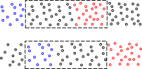
Figure 1: Flow
The purpose of this note is to derive Euler’s equation for fluid flow (equation 19) without cheating, just using sound physics principles such as conservation of mass, conservation of momentum, and the three laws of motion. (There are way too many unsound derivations out there.)
This document is also available in PDF format. You may find this advantageous if your browser has trouble displaying standard HTML math symbols.
To set the stage, consider the example shown in figure 1. The top half is a snapshot of the fluid at some initial time t0 and the bottom half is a snapshot at some slightly later time t1. One parcel of fluid has been marked with blue dye, and another parcel has been marked with red dye. The rectangle represents an imaginary box, also called the “control volume” ... we will be particularly interested in what is happening within this box.
There are some qualitative observations that we can make immediately:
Suppose we have a fluid with local density ρ(t,x,y,x) and local velocity v(t,x,y,z). Consider a control volume V (not necessarily small, not necessarily rectangular) which has boundary S. The total mass in this volume is
| M = | ∫ | ρ dV (1) |
The rate-of-change of this mass is just
| = | ∫ |
| dV (2) |
The only way such change can occur is by stuff flowing across the boundary, so
| = | ∫ | ρ v · dS (3) |
We can change the surface integral into a volume integral using Green’s theorem, to obtain
| = − | ∫ | ∇ · (ρ v) dV (4) |
Compare equation 2 with equation 4. They are equal no matter what volume V we choose, so the integrands must be pointwise equal. This gives us an expression for the local conservation of mass:
| + ∇ · (ρ v) = 0 (5) |
We can understand this expression by referring back to figure 1. At the right edge of the figure, the fluid is relatively dense and has a relatively high velocity, causing a large outflow of fluid from the control volume (the red parcel). At the left edge, the density is relatively low and the velocity is relatively low, causing a small inflow of fluid. The x-derivative of ρ vx is positive. This is the crucial contribution to ∇ · (ρ v); the other two contributions vanish in this example. We have a net outflow of fluid, which causes a decrease in the density of the fluid in the control volume, in accordance with equation 5.
Equation 5 is sometimes called a continuity equation. It is one way to express conservation of mass.
We can go through the same process for momentum instead of mass. We use Π to represent momentum, to avoid conflict with P which represents pressure. The total momentum in the control volume is:
| Πi = | ∫ | ρ vi dV (6) |
where the index i runs over the three components of the momentum. The rate-of-change thereof is just
| = | ∫ |
| dV (7) |
We (temporarily) assume there are no applied forces (i.e. no gravity etc.) and no pressure (e.g. a fluid of non-interacting dust particles). We also assume viscous forces are negligible. Then, the only way a momentum-change can occur is by momentum flowing across the boundary:
| = | ∫ | (ρ vi) v · dS = | ∫ | (ρ vi) vj djS (8) |
We are expressing dot products using the Einstein summation convention, i.e. implied summation over repeated dummy indices, such as j in the previous expression.
We can change the surface integral into a volume integral using Green’s theorem, to obtain
| = − | ∫ | ∇j (ρ vi vj) dV (9) |
Compare equation 7 with equation 9. They are equal no matter what volume V we choose, so the integrands must be pointwise equal. This gives us an expression for the local conservation of momentum:
| = |
| = − ∇j (ρ vi vj) (10) |
We can understand this equation as follows: each component of the momentum-density ρ vi (for each i separately) obeys a local conservation law. There are strong parallels between equation 5 and equation 10.
Note that the ∇j operator on the RHS is differentiating two velocities (vi and vj) only one of which undergoes dot-product summation (namely summation over j). Using vector-component notation (such as ∇jvj) is a bit less elegant than using pure vector notation (such as ∇·v) but in this case it makes things clearer.
We now consider the effect of pressure. It contributes a force on the particles in the control volume, namely
| (11) |
A uniform gravitational field contributes another force, namely
| Fi += | ∫ | ρ gi dV (12) |
These forces contribute to changing the momentum, by the second law of motion:
| = Fi (13) |
Note the tricky notation: we write d/dt rather than ∂/∂t, and Π′ rather than Π, to remind ourselves that the three laws of motion apply to particles, not to the control volume itself. The rate-of-change of Π, the momentum in the control volume, contains the Newtonian contributions (equation 11 and equation 12 via equation 13) plus the flow contributions (equation 10).
Combining all the contributions, we obtain the main result, the equation of motion:
| + ∇j (ρ vi vj) = −∇i P + ρ gi (14) |
Converting from component to notation to vector notation, we get:
| + ∇ (ρ v ⊗ v) = −∇ P + ρ g (15) |
where ⊗ is the tensor product, sometimes called the outer product. (This is not to be confused with the wedge product ∧, which is sometimes called the exterior product.)
As a way of expressing the equation of motion, equation 14 or equivalently equation 15 has many advantages. It has a somewhat elegant symmetrical form. It emphasizes the momentum density ρ v, and expresses conservation of momentum in a way that is strongly analogous to conservation of mass (equation 5). This D=3 expression can readily be generalized to give an expression that is valid in D=1+3 spacetime. It assumes viscous forces are negligible, but it is otherwise rather general.
One sometimes encounters other ways of expressing the same equation of motion. Rather than emphasizing the momentum, we might want to emphasize the velocity. This is not a conserved quantity, but sometimes it is easier to visualize and/or easier to measure. If we expand the LHS we get
| + |
| + vi ∇j (ρ vj) + ρ vj ∇j (vi) = −∇i P + ρ gi (16) |
where the second and third terms cancel because of conservation of mass (equation 5), leaving us with
| ρ |
| + ρ vj ∇j (vi) = −∇i P + ρ gi (17) |
Converting from component notation to vector notation, we get:
| ρ |
| + ρ (v · ∇) v = −∇ P + ρ g (18) |
If we divide through by ρ, we obtain a version of version of Euler’s equation that focuses attention on velocity and acceleration:
| (19) |
This is a famous and important equation. It assumes viscous forces are negligible, but it is otherwise rather general.
It is sometimes convenient to introduce the notion of head, defined as:
| (20) |
The approximation in the second line of equation 20 is valid when the density ρ is approximately constant over the region of interest. (Throughout this document we assume g is constant.) The dot product on the first line contributes a minus sign, because g is directed downwards while dz is directed upwards.
| ρ |
| + ρ (v · ∇) v = −∇ H (21) |
Roughly speaking, we see that the head plays the role of some sort of potential energy. The pressure and the gravitational potential energy contribute equally to the head. The head gives rise to a force on the RHS of equation 21, roughly in accordance with the principle of virtual work.
A few words of warning about equation 18: the first term on the LHS looks reminiscent of the second law of motion: a mass-density times an acceleration. And the RHS looks like a force-density. But that is not a good way to think about it, for reasons that will become clear in a moment. A lot of people who ought to know better (e.g. Landau and Lifschitz) purport to derive Euler’s equation by analogy to the second law. That is, they start with ρ dv / dt, set it equal to the force-density and then correct it with the flow term (the second term on the LHS of equation 18). Alas, that’s logically unsound, and I don’t see any way to fix it. The alternative is to use the correct expression for the force density, i.e. equation 15, which has ρ inside the derivative ∂(ρv)/∂t.
Equation 15 is worth emphasizing. It is useful unto itself, it is easy to remember in analogy to equation 5, and it is a valid starting point for a derivation of the traditional Euler equation. It also has the nice property that, with minor modifications, it can be put in relativistically-correct form.
In this section we will need the definition of vorticity:
| (22) |
We will also need to recall a few properties about wedge products and dot products. For orthonormal vectors x^, y^, and z^:
| (23) |
We will also need the vector identity:
| (24) |
The LHS is |v| times the directional derivative, differentiating along the direction along a streamline. Qualitatively, the first term on the RHS has to do with change in magnitude of v, while the second term has to with change in direction.
We plug that into equation 19 to obtain:
| (25) |
In a simple vortex, the velocity is proportional to 1/|r|. That makes the vorticity zero everywhere except at the origin. If we assume steady flow and uniform density, we can integrate equation 25 to obtain:
| (26) |
which means the lowest pressure is in the center, where the speed is highest. In this case, lower pressure is associated with higher velocity.
Next we consider fluid undergoing uniform rotation, i.e. velocity proportional to r. Then the vorticity is everywhere constant, equal to 2ω times a unit bivector in the plane of rotation, where ω is the angular rate of rotation. The −Ω·v term is twice as large as the ∇(½v2) term and in the opposite direction.
| (27) |
Once again the lowest pressure is in the center. However, quite unlike equation 26, in this case lower pressure is associated with lower velocity.
In both cases, and much more generally, whenever the streamlines are curved there will be lower pressure on the inside of the turn. This is easy to understand, even without using Euler’s equation. We assume steady flow, and more-or-less constant density. At some location the fluid is moving with velocity v along a streamline with radius of curvature r. Then the local acceleration is v2/r, in accordance with the most basic laws of motion. The pressure gradient is then ρv2/r, with lower pressure on the inside of the turn.
Note the asymmetry in equation 25:
| As discussed in section 4, when we integrate along a stream line, the ∇(½v2) term is the one that matters. | When we integrate in a direction across the streamlines, both the −Ω·v and the ∇(½v2) terms contribute. |
To derive Bernoulli’s formula, we assume steady flow and approximately constant density, and then integrate equation 25 along a streamline.
Because the flow is steady, the time derivative on the LHS of the equation vanishes.
Because we are integrating along a streamline, the term involving Ω∧v drops out. That’s because it is a vector directed crosswise to the streamline. Note that for any bivector B whatsoever,
| (28) |
In our case the bivector is ∇∧v, but equation 28 holds more generally.
We integrate from point B (“before”) to point A (“after”) along a streamline:
| ∫ |
| (½ρ∇ (v·v) + ∇ H)·ds = 0 (29) |
We want to move ρ outside the integral, so we assume that point B and point A are not too far apart, and that ρ is slowly varying. You can quantify this by expanding ρ in a power series as a function of pressure, and keeping only the zeroth order term. (The higher-order terms allow you to estimate the accuracy of the approximation.)
Equation 30 is the “baby Bernoulli” formula. More sophisticated versions of this formula can be derived, for instance versions that relax the assumption about constant density. See reference 2, reference 3, and reference 4.
In some situations the ρ|g|z term on the RHS of equation 30b can be neglected. This makes sense when the velocity is sufficiently large and the region of interest is sufficiently limited in the z direction. This is commonly the case when considering the flow of air over a wing, or the flow of air through a carburetor. On the other hand, there are situations where the ρ|g|z term must be retained, including any situation where buoyancy is significant.
It must be emphasized that equation 30 is only valid for a parcel of fluid moving along a particular streamline. In particular, the constant on the RHS may be (and often is) different for different streamlines.
In steady flow, you can compare different parcels along the same streamline, because they are essentially earlier and later versions of the same parcel. However, Bernoulli’s principle (by itself) does not let you compare one streamline with another.
This is a serious restriction, because in any situation where you want to calculate the lift, you want to compare the pressure along one streamline with the pressure along another. Bernoulli’s equation by itself cannot do this. Sometimes you can make progress by combining Bernoulli’s equation with some other information, and sometimes you can’t.
Sometimes, in some special case, you may be able to ascertain that the constant in equation 30 for one streamline bears some simple relationship to the constant for another streamline. The two constants may even be equal, in which case you can conclude that ½ρv2 + H has the same value for those two streamlines. Just remember that this is not the general case. See reference 2.
In particular, even though equation 26 is consistent with equation 30b, it cannot be derived by application of Bernoulli’s principle alone. Any such derivation would be a swindle, as we can see from the fact that the same approach would get the completely wrong answer in equation 27.