|
| |
| Figure 1: Unstretched O-Ring | Figure 2: Basic Notion of Force-Application | |
:
Our first goal is to paint a simple yet uncompromisingly correct picture of what we mean by force. We start with a constructive, operational definition of force in a particular situation (figure 2) ... and we then explain which aspects of this situation generalize to all forces, and which do not.
The second goal is to explain the relationships between force and momentum. Many questions that are asked in terms of force are best answered in terms of momentum. We shall see that the so-called three laws of motion can all be understood as corollaries of conservation of momentum. See section 4.2.
The third goal is to explain how force and momentum are related to torque and angular momentum.
The first few weeks of the introductory physics course focus on the mechanical motion of individual, concrete, tangible particles. That’s fine as a starting point, but not as an ending point. Eventually it is necessary to move on to a higher level of abstraction.
Basic idea #1: Force is a vector. That means it has direction and magnitude. For details on what we mean by vector, see reference 1.
Basic idea #2: Force is a well-defined physical quantity. We have ways of measuring the force. We can measure the direction and magnitude.
Tangential remark: The idea of force is intertwined with some other ideas in ways that will be explained in section 5.
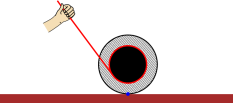
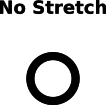
The following diagrams provide some simple, easy-to-visualize forces. Our basic approach is borrowed from reference 4. In figure 1, there is a plain rubber O-ring in its normal unstretched state.
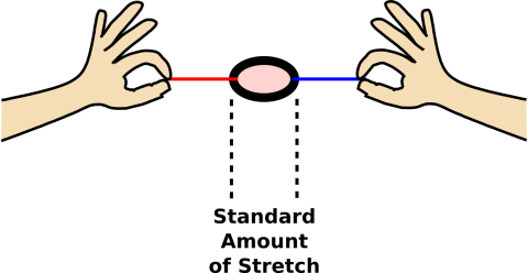
Meanwhile, in figure 2, we are using two strings to pull on the O-ring. The O-ring is acting as a simple type of spring.1 There are several forces involved here. Starting with your left hand and proceeding clockwise, we have:
For present purposes, we assume gravitational forces are negligible.
We have arranged it so that in this situation, each of the four objects involved is subject to one leftward force and one rightward force of equal magnitude. This means all the forces are balanced, in this situation. Unbalanced forces are discussed in section 3.2.
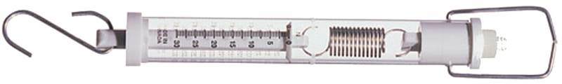
Note that the idea of quantifying force by means of a standardized spring is by no means a silly idea. Figure 3 shows a practical, commercially-available scale that works on this principle. It is more complicated than our stretched O-ring, and more versatile, but it uses the same basic principle.
If you want three times the force, you need to hook up the springs in parallel, as shown in figure 4.
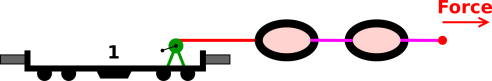
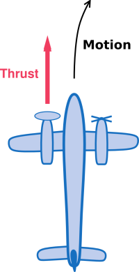
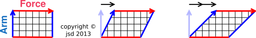
According to any modern definition, force is a vector. Like any vector, any force has a direction and magnitude. Like any vector, it can be represented graphically by an arrow with a tip and a tail. One of the forces in the train situation is shown in figure 5.
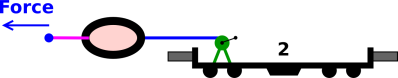
Another of the forces in the train situation is shown in figure 6.
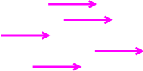
Again: a vector can be represented graphically by an arrow with a tip and a tail. One thing a vector does not have is a location. All five of the arrows in figure 7 represent the exact same vector, because they all have the same direction and magnitude. However, this is not the whole story; physics involves more than just force-vectors, as discussed in section 5.
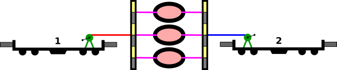
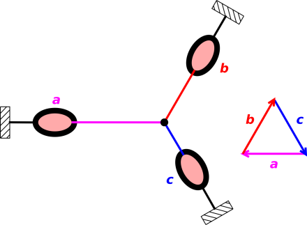
Vectors can be added graphically, tip-to-tail. For example, the net force on the black dot in the center of figure 8 is zero, because the three force vectors add up to zero. Note that the direction of each force can be inferred from the direction of the string, but the magnitude of the force cannot be inferred from the length of the string. The magnitude of each force can be inferred from the amount of stretch in the O-rings, which is the same for all three forces.
In figure 8 and elsewhere in this document, the small black rectangles with diagonal hash-marks represent anchors. They are attached to the earth. We assume that the earth is both rigid and extremely massive. Because it is rigid, it can transmit force from place to place. Because it is massive, it can absorb enormous amounts of momentum without picking up any appreciable velocity, so we consider the position of each anchor to be unchanging. In figure 8 the earth doesn’t pick up any net momentum anyway, because whatever momentum flows into the earth via one anchor is cancelled by flows into the other anchors.
Since force is a vector, we know that the sum of any two forces is itself a force. This is required by the axioms that define what we mean by “vector“; see e.g. reference 5.
Included in figure 8 is a triangular diagram showing that the three forces add to zero. You can understand the addition by adding the three vectors geometrically, tip-to-tail, in the usual way. Start at any corner, add all three vectors geometrically, and you get back to where you started from. You get back to where you started, which is the same as nothing, i.e. zero force.
We also need to check that this triangle correctly represents the physics of the situation. Here is the correspondence:
| In the left part of the diagram, the strings are color-coded: red, blue, and magenta. | The arrows in the force diagram use the same color code: red, blue, and magenta. |
| The orientation of each string tells you the direction of the force. | The orientation of each force-vector matches the orientation of the corresponding string. |
| However, the length of the string tells you nothing about the magnitude of the force. You have to look at the amount of stretch in the O-ring to ascertain the magnitude of the force. In fact all three O-rings are stretched the same amount. | In a vector diagram, the length of the vector indicates the magnitude of the force. In fact all three of our vectors have the same length, as they should. |
The fact that the strings are arranged in a Y-shape while the force-vectors are arranged in a Δ shape is irrelevant. Note the contrast:
We now introduce the idea of a simple pairwise force. Note the contrast:
| Not all forces are simple pairwise forces. About half of this section will be spent warning about things you cannot do with pairwise forces. | Sometimes you do encounter simple pairwise forces, and there are useful things you can do with them. They played an important role in the early days of modern science, in the days of Galileo and Newton, so it wouldn’t hurt to take a look at some examples. |
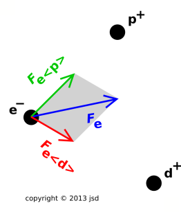
In figure 9, the green force Fe<p> is an example of a simple pairwise force. It is the force exerted on the electron (e−) by the proton (p+) in accordance with Coulomb’s law. (In this section we assume small distances and long timescales, so this is an electrostatic situation, and we don’t need to worry about special relativity.)
In any situation, if we analyze things in enough detail, the total electrostatic force on any given particle can be written as the sum of all the simple pairwise forces that act on that particle. (This may or may not be the smart way to do things, but it’s always possible.) For the electron in figure 9, the total force (Fe) is represented by the blue vector:
| (1) |
As discussed in section 3, there is a reason why forces occur in pairs. For every force Fe<p>, there will be another force Fp<e>, and these forces will be equal-and-opposite. We can express the idea mathematically:
| (2) |
We now introduce some useful terminology, namely the “feeler-dealer” terminology: We say Fe<p> is the force “felt” by the electron “dealt” by the proton. This is entirely equivalent to saying Fe<p> is the force exerted on the electron by the proton, just more colorful.
Not all forces are simple pairwise forces; for example, the total force Fe is not. A force that is not a simple pairwise force could be called a compound force, but usually it isn’t worth the trouble to distinguish compound forces from forces in general. The set of all forces is closed under addition, whereas the set of all simple pairwise forces is not. Recall that closure is required by the vector-space axioms, so the set of all simple pairwise forces is not a vector space. This is one reason why we should not become too enamored of simple pairwise forces.
| Simple Pairwise Forces | Forces in General |
| Equation 2 is a watered-down corollary of the third law of motion. It applies only to simple pairwise forces. | The real third law applies to forces in general. It is conventionally stated in archaic terms as “for every action there is an equal and opposite reaction” but really it is a statement about forces. |
| For example, in figure 9 we cannot find any tangible object that is subject to a force equal-and-opposite to Fe. | The real third law guarantees that some force equal-and-opposite to Fe exists. The counterpart to Fe is not the force on any particular object, but still it is a perfectly good force, namely the sum of Fp<e> plus Fd<e>. |
Also, as a partly-similar, partly-separate idea, note that sometimes the forces involve fields, not just tangible objects, as discussed in section 3.4.
If you want to be even more meticulous and sophisticated, the best approach is to speak of the force exerted on everything in one region of space by everything in some other region of space. See figure 20 and the associated discussion.
If there are N objects, it is always possible to tabulate the simple pairwise forces in the form of an N×N matrix. The restricted version of the third law of motion (equation 2) guarantees that it is an antisymmetric matrix.
| ⎡ ⎢ ⎢ ⎣ |
| ⎤ ⎥ ⎥ ⎦ | (3) |
In general there will be N(N−1) simple pairwise forces, assuming each object interacts with each of the others. The third law tells us these can be grouped into N(N−1)/2 force-pairs.
The total force on a given object is found by summing the appropriate row in the matrix, summing across all columns in accordance with equation 1. One could imagine calculating the corresponding sum along a given column, summing over rows, but this is not recommended. According to 350 years of physics tradition, we focus attention on the force exerted ON the object; this is the force that appears in expressions such as F=ma (the second law of motion). For this reason, in my notation the “dealer” subscript is shown in <⋯> pointy brackets while the “feeler” is not bracketed. Also it is no accident that the brackets point away from the dealer.
The appropriate level of detail is context-dependent:
| Sometimes we are interested mainly in the third law, i.e. in conservation of momentum. In such cases we care about which object dealt the force and which object felt the force. | Sometimes we are interested mainly in the second law. In such cases we care about the total force felt by the object, and we may be completely uninterested in which objects dealt the force. |
Tangential technical note: Figure 9 is slightly incomplete insofar as we consider only the tangible objects and not the fields. However, in this situation, worrying about the details of the fields wouldn’t change the answer. In any electrostatic situation, the fields transmit the forces without change. Contrasting situations are discussed in section 3.4.
Feel free to skip this section. To a first approximations, beginners should not spend time worrying about misconceptions. It is more important to understand what a force is – or at least what it does – rather than worrying about all the things that force isn’t.
However, in some cases it may be helpful to briefly mention the following points:
For an object going around a turn, the motion is in one direction and the force is in another.
For example, suppose two persons of the same size and mass (Bob and Charlie) are facing each other on ice skates. (We choose ice skates because they provide famously low friction.) Bob pushes on Charlie, and the two go flying apart. So a certain amount of force was exerted on Charlie. How much force was exerted on Bob?
In physics terms, the force on Bob is equal-and-opposite to the force on Charlie. This illustrates the difference between physics terms and homespun terms. The homespun force has to do with causation and volition, and all of that belongs to Bob – not Charlie – in this scenario. In contrast, physics force is a measurable thing. According to every measurement that has ever been done, the force acting on Bob is equal-and-opposite to the force acting on Charlie in this situation, which is what we expect based on the third law.
If this runs contrary to your previous understanding of the word force, you’ll just have to recognize that physics context is different from homespun context. In physics, we assign a very specific technical meaning to the word force. That’s OK; most English words have multiple meanings. You don’t have to unlearn the other meanings, but you must recognize that they don’t apply in physics context. A lap in the swimming pool is conceptually different from a lap on the racetrack. Organic chemistry has little to do with organic farming. Closing a switch for electricity is functionally the opposite of closing a valve for fluids. For more examples if this kind, see reference 6. Context matters. Get used to it.
The same goes for other physics terms. There’s a long list: force, momentum, energy, elasticity, conservation, et cetera. In physics context, be sure to use the physics definition.
If you are interested in cause-and-effect (as opposed to force), see reference 7.
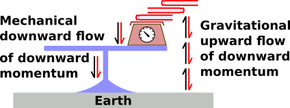
Let’s consider the situation shown in figure 10. A stack of books is sitting on a scale, which sits on a table, which sits on the ground. This is the ordinary situation, where everything is in mechanical equilibrium. That is to say, all the forces are in balance.
We can understand this in terms of momentum flow:
Momentum-flow is represented by a double arrow, with two half-arrowheads. The colored part of the arrow shows what is flowing, while the black part of the arrow shows in which direction it is flowing.
It is characteristic of an equilibrium situation that we have a closed circuit of momentum flow. The momentum flows around and around, without any net accumulation anywhere.
This idea – closed-circuit flow with no accumulation – is similar to the first law of motion, only stronger: no net force means no change in momentum.
(For simplicity we have not considered the weight of the table itself; you can easily add that to the picture you want.)
In my experience, most people don’t have a problem with the idea of conservation when there is flow without accumulation. They have a pretty good intuition about continuity of flow in a loop. If anybody isn’t happy with this, put some water in a big round bowl and stir up a steady rotational flow. The water is conserved. The water is flowing, but for steady flow there is no accumulation anywhere.
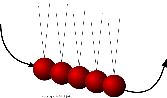
Figure 11 shows my favorite demonstration of momentum flow. Balls #2 through #5 are initially at rest. Ball #1 swings in from the left. Momentum leaves ball #1 and flows through balls #2, #3, and #4 without accumulating. It accumulates in ball #5, which goes flying.
Figure 12 shows a video of such a thing in action: (Video courtesy of GiantNewtonsCradle.com.)
Trying to analyze this in terms of forces would be tricky. A reasonable amount of momentum is transfered in near-zero time, which leads to a near-infinite force.
Tangential remark: The usual Newton’s cradle apparatus has a special property that is often overlooked: At rest, the balls are not touching; there is a paper-thin air gap. Therefore when ball #1 arrives, there is not a single collision, but rather a rapid sequence of collisions.
There is a good physics reason for this:
| During an elastic collision between one ball and one other, conservation of momentum and conservation of energy give us two equations in two unknowns, so we can predict what happens. We can then understand the next collision, and proceed by induction. | If ball #1 interacted with the other four balls all at once, we would have two equations in five unknowns, and there would be innumerable possible outcomes, all consistent with the laws of physics. |
For more on this, see reference 8 and references therein.
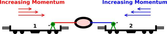
Figure 13 shows a situation where some of the forces are not in balance. Specifically, the forces on the O-ring are balanced, but the forces on the model train cars are not. We assume that the trains have really good bearings, so that any frictional forces are negligible. The only force on the train cars comes via the strings.
For simplicity, we assume there is a winch on board each train. We use the winches to stretch the O-ring to the standard shape, so that it provides the standard amount of force. This is tricky to do when the train is moving, but we assume it is done properly. The details of how it is done are not important for present purposes. Note: Whenever an O-ring is stretched by the standard amount, we show it filled with a pink background color. In the real world, O-rings do not change color like this, but we use this representation to make the diagrams easier to understand.
The smart way to think about situations like this is in terms of momentum. If a force is acting on a system, it changes the momentum according to the following rule:
| (4) |
Compare equation 7.
Force is a vector, and momentum is a vector.
Momentum is truly fundamental. It sits right at the core of what we call physics. Momentum is conserved, everywhere, always. For details on what we mean by conservation, see reference 3.
In figure 13 and many of the other figures in this document are snapshots of a dynamic situation. It would be better to use a movie, to show explicitly that the momentum of each train is changing. However, making movies is a tremendous amount of work, and I haven’t gotten around to it. In these figures, whenever you see a group of three arrows of different length, think of it as three successive snapshots of the same vector, indicating that the vector is changing over time. Within such a group, the earliest vector is on top, and the latest vector is on the bottom.
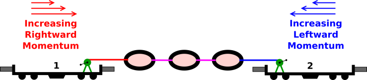
In figure 14, we have hooked up three springs in series. It must be emphasized that the forces in this situation have the same magnitude as in figure 2; we definitely do not get a three-times-larger force. The smart way to think about this is in terms of momentum flow.
In physics, as in every part of everyday life, it is important to look at things from more than one viewpoint. We shall see that force and momentum-flow are two nearly-synonymous ways of describing the same physics. In some situations, the force concept is more useful, but in other situations the momentum-flow concept is more useful. In favorable situations, you can describe things either way, and each serves as a check on the other, greatly increasing the reliability of the conclusions.
At this point, you should take a moment to make sure you understand continuity of flow of a scalar quantity, such as the flow of water,2 the flow of energy, or the flow of electrical charge. See reference 2 and reference 3. This is a prerequisite for understanding the flow of more complicated things. As a next step, consider the flow of one component of momentum, such as the x-component, i.e. p·x, for some fixed x.
Energy is a scalar. The flow of energy is a vector.
Charge is a scalar. The flow of charge (i.e. the current) is a vector.
The x-component of momentum is a scalar. The flow of p·x is a vector.
More generally, the full momentum p is a vector. The flow of p is a symmetric second-rank tensor, namely the stress tensor. In any chosen basis, it cann be represented by a symmetric 3×3 matrix. The stress tensor is not particularly easy to visualize. However, we don’t need to worry about it right now, especially when considering the motion of a train that is constrained to move in one dimension. For present purposes, and a lot of other purposes besides, it suffices to keep track of the momentum flow on a component-by-component basis.
In figure 14, the same momentum flows through all three springs. If you hook three garden hoses end-to-end, you do not get three times as much water. The same water flows through all three hoses.
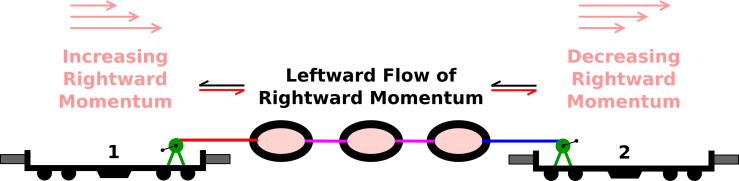
Train #1 will gradually accumulate rightward momentum, and train #2 will gradually accumulate leftward momentum. In train #1, the increase in rightward momentum is synonymous with a decrease in leftward momentum. Momentum is a conserved quantity, so the only way that leftward momentum can disappear from train #1 and appear in train #2 is by flowing from one to the other, by flowing through the strings and springs.
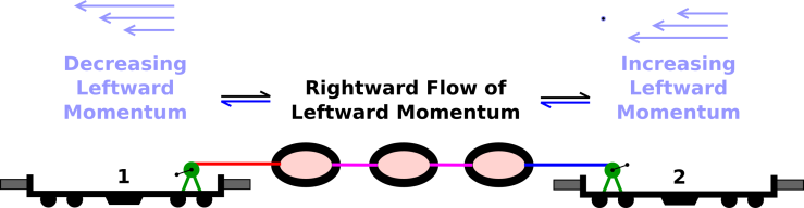
In figure 15, we emphasize the flow. As before, this is shown by a double arrow, with two half-arrowheads. The colored part of the arrow shows what is flowing (namely leftward momentum), while the black part of the arrow shows in which direction it is flowing (namely rightward).
Equivalently, you can describe the situation in terms of rightward momentum flowing out of train #2 and accumulating in train #1, as in figure 16. Again flow is represented by a double arrow. The colored part of the arrow shows what is flowing (namely rightward momentum) and the black part of the arrow shows in which direction it is flowing (namely leftward).
The double arrows communicate an important idea: Momentum-flow is not a vector. In particular, the tension in a string is not a vector. Note the contrast:
| If you rotate a vector 180∘ (in a plane containing the vector), you get the opposite vector. | If you rotate a string 180∘ (in a plane containing the string) you get an equivalent situation with the same tension. |
| Momentum is a vector. | Momentum-flow is not a vector; it is a second-rank tensor. |
If you want to get technical about it, the tension in a string is the outer product of two vectors. On the other hand, if the previous sentence didn’t mean anything to you, don’t worry about it.
The idea of momentum flow gives us a nice way to understand that all three springs must be stretched the same amount. You can see that the same amount of momentum is flowing through each spring. Momentum is conserved, and no momentum is accumulating in the springs or strings. No momentum accumulates in the strings or springs, because in this situation it flows out as fast as it flows in.
If you want to get three times the force, you need three springs in parallel, as in figure 4.
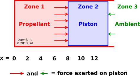
In this section we consider an air gun, as shown in figure 17. Zone 1 contains some pressurized gas (the propellant). Zone 2 is the piston. Zone 3 is the ambient atmosphere.
The system starts out at rest, with the piston at x=1. (We measure the position of the piston by the location of its left edge, since that is what determines the volume available to the propellant.) Then at t=0 we release the piston. The propellant expands. The diagrams in this section are a snapshot of the situation at some later time.
The forces exerted ON the piston are indicated by the arrows in figure 17.
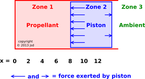
Meanwhile, we can also ask about the forces exerted BY the piston; these are indicated by the arrows in figure 18.
By comparing figure 17 with figure 18 we can verify that the third law of motion is upheld: Momentum flow across a boundary gives rise to a pair of simple pairwise forces. For every force exerted on A by B there is an equal-and-opposite force exerted on B by A.
If this were a fluid-dynamics task, Zone 2 would not be a rigid piston; it would just be another parcel of gas. We would have one parcel of gas pushing on another, which pushes on another, et cetera.
In such a situation, it makes sense to talk about the pressure at a particular location, such as the pressure at x=8 in figure 18. However, it is hopelessly confusing to talk about “the” force at x=8, because nobody knows whether you are talking about the rightward force in figure 17 or the rightward force in figure 18.
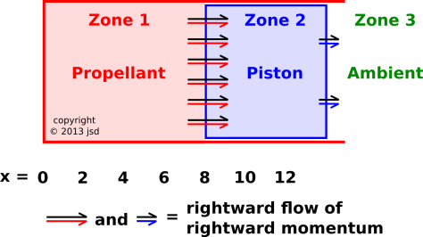
The smart way to proceed is to reformulate things in terms of momentum flow. This works for a huge range of tasks, from the very simple to the very complex. There is a perfectly well defined boundary at x=8, and we can unambiguously talk about the momentum flowing across this boundary. This is shown in figure 19. As in section 3.2.2, we represent momentum flow by a double arrow: The black part of the arrow indicates the direction of flow (namely rightward), while the colored part indicates what is flowing (namely rightward momentum).
As you might imagine, rightward flow of rightward momentum is synonymous with leftward flow of leftward momentum. We will not bother to diagram the latter, because in our air gun all the relevant momenta are rightward. However, it is worth noting that pressure is not a vector. If you rotate a vector 180∘ (in a plane containing the vector) you get the opposite vector. In contrast, if you rotate a pressurized fluid (by any amount, in any direction) you get the same pressure. In fact, pressure is a scalar.
By formulating the task in terms of momentum flow, we get the third law of motion for free. The law is upheld automatically. The momentum flowing from A to B is synonymous with the momentum flowing from B to A. We’re not merely saying that the two momenta are numerically equal; we’re saying it is the same momentum. A particular batch of momentum is moving from one place to another.
In figure 19 you can see that rightward momentum is flowing into the piston faster than it is flowing out. That means that over time, momentum will accumulate in the piston.
This allows us to understand the second law of motion. We can see it as compatible with other things we know, indeed as a consequence of other things we know, as follows:
The first two items taken together imply the second law of motion. The third item guarantees that the law is meaningful and non-tautological. That is, we are not relying on the second law to define what we mean by force. (If we did that, you would have to wonder whether the whole argment was circular.)
For a discussion of some misconceptions pertaining to this air gun, see reference 9.
As always, the law of conservation of momentum can be expressed as an equation:
| (5) |
This law applies to the momentum vector as a whole, which means that a similar law applies to the x, y and z components separately. Each component is separately conserved. The law applies to every region of space, no matter how large or small. For details on this, see reference 3.
Let’s focus attention on a particular piece of momentum flow, such as the flow from region B to region E in figure 20. Conservation means that the momentum that flows from B to E is exactly the same as the momentum that flows to E from B. I’m not just saying these two things are numerically equal; I’m saying it is the very same momentum. It disappears from region B and appears in region E. Furthermore, we can also say that the momentum that flows from B to E is the negative of the momentum that flows the other way, from E to B. That’s just two ways of saying the same thing.
The flow from E to B is not in addition to the flow in the other direction. There is only one flow. The point is that we have several different sets of words for describing the same flow. Some momentum is disappearing from region B and appearing in region E.
If we translate this idea to the language of forces, we get the third law of motion: The force that B exerts on E is equal-and-opposite to the force the E exerts on B. So we see that the third law of motion is a corollary to the law of conservation of momentum. Expressing the idea in terms of conservation is slightly more powerful.
Of course there can be other forces, i.e. other momentum-flows, such as a flow from B to A or from B to C. However, if we restrict attention to the direct interaction between B and E, conservation tells us that whatever momentum crosses the boundary from B to E must simultaneously be lost from B and gained by E. This is absolutely exact, guaranteed.
Suppose we are interested in the dynamics of region B. Common sense tells us that to solve the whole problem, we need to calculate the entire force on the region. We need to calculate the entire momentum-flow into the region. This is as it should be. On the other hand, there is a proverb that says a journey of 100 miles begins with a single step. In many cases, there is a tactical advantage to calculating the momentum flow across some small part of the boundary of region B, such as the part that abuts region E. The conservation idea can help us do this part of the calculation. During this step, we should not allow ourself to be distracted by what’s going on elsewhere. Later, we can repeat the process for all other parts of the boundary. Finally, we add up all the partial results, to find the total momentum flowing into region B.
Consider the following contrast:
| Initial Step | Eventual Goal |
| Part of the force on B, namely the force that E exerts on B. | The total force on B (and perhaps the total force on E). |
| Momentum is always strictly conserved, in accordance with equation 5. | Momentum is always strictly conserved, in accordance with equation 5. |
| As a corollary, we can describe this part of the situation in 17th-century terms: action accompanied by equal-and-opposite reaction. | The 17th-century approach is often not directly applicable to the overall situation, or not convenient, especially when there are complicated N-way interactions. In particular: The total force on B is not necessarily equal-and-opposite to the total force on E. |
| The modern approach always works: Momentum is always strictly conserved, in accordance with equation 5. Conservation applies to region B as a whole, to region E as a whole, and to each and every part of the boundary, including the E/B boundary. |
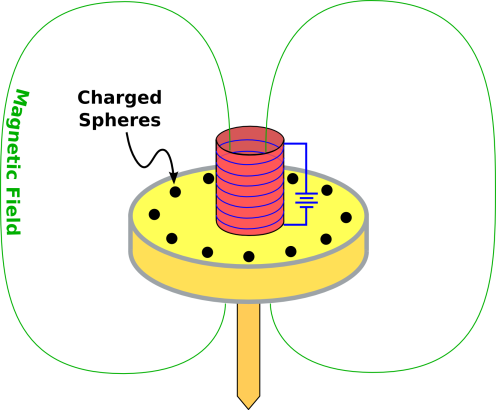
Consider the apparatus shown in figure 21, which is based on figure 17-5 in Feynman volume II; see reference 10. The device is initially at rest. A number of small charged spheres are mounted on an insulating disk. A current is flowing in the solenoid, creating a magnetic field. If we cut off the current, the magnetic field goes to zero. The changing magnetic field will create a force on the charged spheres, causing the disk to spin on its axis.
In section 17-4, Feynman asks, where does the angular momentum come from? The answer is given at the end of section 27-6: In general, there is momentum in the electromagnetic field. When we cut off the current in figure 21, the momentum is transferred from the electromagnetic field to the mechanical parts of the apparatus.
The idea of fields is also relevant to the simple situation shown in figure 9. Rather than considering just the three tangible objects, it would be more accurate to consider the electromagnetic field also. The proton interacts with the field, and then the field carries the interaction from place to place, and finally the field interacts with the electron. Similar words apply to the other interactions. The concept of field allows us to interpret the third law properly, so that it applies “right here, right now” – i.e. locally at each and every point in spacetime. In other words, there is no such thing as action at a distance. However, in the nonrelativistic limit, the field carries the interaction from place to place almost instantaneously, so everything we said in section 2.3 is true to an excellent approximation.
For that matter, according to any modern (post-1924) understanding of physics, everything is a field. For example, the electron in figure 9 is an excitation in a certain fermionic field. So really, any force whatsoever is just transferring momentum from one field to another.
In any case, the momentum-flow viewpoint always gets things right, with or without the nonrelativistic approximation.
The law of conservation of momentum can be seen as a corollary of conservation of angular momentum, as follows: Angular momentum is conserved no matter what pivot point you choose. If you a pivot point infinitely far away in the X direction, there is no way to conserve angular momentum unless plain old linear momentum is conserved, with the possible exception of the X-component of momentum. If you choose three non-colinear pivot points, then you can prove that linear momentum must be conserved, with no exceptions, as a consequence of conservation of angular momentum.
The three laws of motion are conventionally (if not wisely) written as follows:
Tangential remark: This was published by Galileo in 1638, many decades before Newton came on the scene. Furthermore, it can be seen as a corollary of Galileo’s principle of relativity. Therefore, calling this “Newton’s” first law would be quite strange. Newton gets credit for putting this law at the top of a numbered list, but he did not originate the law. It’s Galileo’s law, not Newton’s.
Beware: The conventional statement in the previous sentence is OK for zero-sized particles, but for an extended object or system it is very incomplete, because it doesn’t say anything about the line of application.
The point of this section is that all three laws of motion can be best understood as corollaries of the law of conservation of momentum, equation 5, which we restate here:
| (6) |
We can unify, simplify, and clarify the laws of motion as follows:
If we look at the full four-dimensional momentum in spacetime, we find that if the momentum is constant, then the mass is constant. For details on this, see reference 11.
Finally, if we divide the constant momentum by the constant mass, we find that the velocity is constant.
Bottom line: As advertised, we have recovered the first law as a corollary of conservation of momentum, for an isolated system.
This is a very useful corollary, because there are many cases where we can calculate the force directly, such as the force due to the electromagnetic field, the gravitational field, or the standard force defined by figure 2.
However, this is not the whole story, because a force is not the only way to transfer momentum across a boundary. The other possibility is advection. Suppose you choose your “system” to be a region of space containing some dust. Now some additional dust crosses the boundary of your system. The momentum of the new dust now contributes to the momentum of the system, even though no force has been exerted.
Bottom line: We see that the conventional second law is a corollary of conservation of momentum, applicable when there is no advection, and useful when we have a way of knowing the force.
We can restate this result in terms of force if we ignore advection and equate force with momentum per unit time. We now invoke the fundamental theorem of calculus: Since the momentum-transfer has to be equal-and-opposite over each and every time interval, the instantaneous force has to be equal-and-opposite.
In special relativity, the idea of conservation of momentum is absolutely clear and easy to use. Translating this to the language of forces is slightly trickier, because it requires dividing by time, and the time-axis in one frame might be rotated relative to the time-axis in another frame. When in doubt, formulate things in terms of momentum, not force.
It would be possible to develop a notion of force independent of momentum and conservation of momentum, but that is not recommended.
It is a good investment to learn about conservation, because you get to use the idea over and over again.
There are some interesting exceptions to this rule, for instance having to do with the synthesis of radioactive FDG for use in medical PET scans. You actually have to hurry the chemistry, and then use the FDG promptly, because the half-life of the man-made 18F is only about 108.9 minutes.
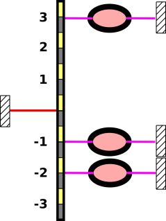
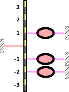
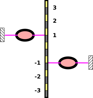
| In figure 22, I assert that the forces are in balance and the torques are in balance. We shall see how to quantify this in a moment; see equation 8. Even if we don’t know the torque, we can immediately surmise that in this figure, the tension in the red string is three units of force. | In figure 23, I assert that the forces are in balance but the torques are not in balance. The forces are exactly the same as in the previous figure, but the strings are pulling in different places. The strings have different amounts of leverage. The gray-and-yellow bar will immediately start to rotate. Its center of mass will not move (assuming it was initially at rest) since the net force is zero, but the bar will rotate around its center of mass at an ever-increasing rate. |
Torque is related to angular momentum in the same way that force is related to momentum. If a torque is acting on a system, it changes the angular momentum according to the following rule:
| (7) |
Compare equation 4.
Angular momentum is conserved. It obeys the same sort of strict local conservation law as other conserved quantities such as charge, energy, momentum, lepton number, et cetera.
To calculate the torque, you need to know the force and the lever-arm. The amount of torque is defined by the following formula:
| (8) |
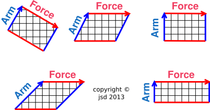
where the arm (also called lever arm) is a vector representing the separation between the pivot-point3 and the point where the force is applied. In this formula, we are multiplying4 vectors using the geometric wedge product, denoted “∧”. The wedge product of two vectors is called a bivector, and is represented by an area, namely the area of the parallelogram spanned by the two vectors, as shown in figure 24. All five bivectors in the figure are equivalent, as you can confirm by counting squares.
| A scalar has no geometric extent. It is zero-dimensional, and is drawn as a point with no size. |
| A vector (such as force) has geometric extent in one dimension. The drawing of a vector has a certain length. | A bivector (such as torque) has geometric extent in two dimensions. The drawing of a bivector has a certain area. In particular, the torque in figure 23 is represented by an area in the plane of the paper. |
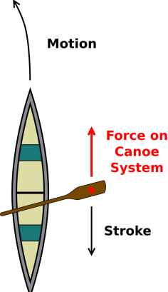
Consider the canoeing situation shown in figure 25. We define the canoe plus canoeist plus paddle to be “the system” for present purposes. Initially the system is at rest. Then a force in the forward direction is applied to the system via a paddle that sticks out to the right of the canoe. The point of application is shown in the figure by the red dot on the paddle. This is the only point where significant momentum is entering the system in the short term.5 We expect the canoe to move forward and yaw to the left.
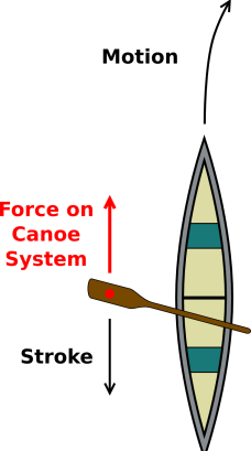
In contrast, in figure 26, a force in the forward direction is applied to the system via a paddle that sticks out to the left of the canoe. We expect the canoe to move forward and yaw to the right.
It must be emphasized that the force is the same in both of these situations. However, the overall physics of the situation is the different. Force is not the whole story.
We therefore introduce the idea of dynamic interaction:
The point of application does not “belong” to the force, nor vice versa. They both “belong” to the interaction.
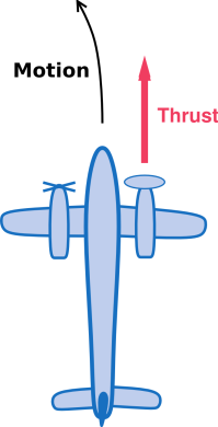
Another real-world example of a dynamic interaction is shown in figure 27 and figure 28.
The physics in figure 27 is very different from the physics in figure 28, even though the force is the same. The point of application is different.
Familiar examples of a dynamic interaction include a push, a pull, or a shear. (Shear is discussed in section 7.)
In this context the position vector is called the lever arm.
Only the component of the lever arm perpendicular to the force contributes to the torque, as discussed in section 6.4. Therefore a slightly more abstract way of specifying the forque is to specify the force and a point in a plane perpendicular to the force. This representation has the advantage that it doesn’t require choosing a datum.
Equivalently, we can think in terms of the line that runs parallel to the force and passes through the point of application. This is called the line of action.
In any case, the forque tells us about the transfer of momentum and angular momentum.
Only the component of r parallel to the force contributes to the work.
| (9) |
Equivalently, it suffices to keep track of F and all components of r.
These representations have various advantages and disadvantages as discussed in section 6.3.
Figure 29 shows an example of a simple problem where the idea of line of action provides some insight, and provides a simple method of solution. A yo-yo rolls without slipping on the tabletop. The question is, when I pull on the string, will it roll to the left, or roll to the right?
On the other hand, figure 30 shows a forque where there is a torque, but no net force. We can describe the overall change in momentum in terms of an overall force, and we can describe the overally change in angular momentum in terms of a torque ... but we cannot describe the situation in terms of a force and point of application.
In this situation the idea of point of application (or line of action) of the “overall” force fails miserable. It is undefined and undefineable. Obviously you can describe the situation in terms of two forces and two points of application, but they cannot be combined.
Various ways of representing a forque are discussed in section 6.3.
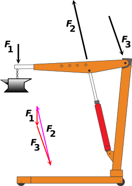
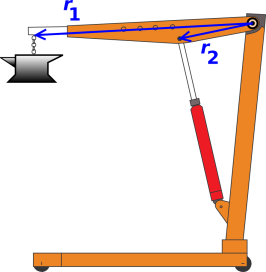
Let’s apply the forque idea to a hydraulic shop crane, as shown in figure 31 and figure 32. We use the symbol χ (Greek letter chi) to represent a forque. There are three main forques affecting the boom:
For simplicity, we ignore the weight of the boom itself. Similarly, we ignore the weight of the hydraulic cylinder, which makes it much easier to figure out the direction of F2. Feel free to re-do the problem including these contributions, if you want.
Figure 31 makes use of the fact that a vector has a magnitude and a direction but not a location. We draw each force vector twice, once in black and once in red or magenta. We locate the each black arrow somewhere near the point of application of the forque. Meanwhile, we locate the red and magenta arrows in such a way as to demonstrate that the three forces add up to zero, as they should in an equilibrium situation.
Figure 32 shows the lever arms for each forque. We choose the datum to coincide with the shoulder joint, as indicated by the ⊙ symbol. This is a convenient choice, because it guarantees that the r3 lever arm is zero.
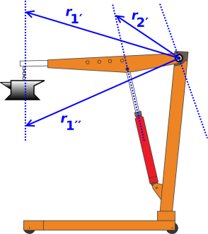
An interesting wrinkle is shown in figure 33. The vertical dotted blue line is parallel to F1. That means we can describe forque χ1 equally well using any of the three lever arms r1, r1′, and r1″. The lever arms are different, but the forque is the same, because the forque only cares about the force and the torque. The torque is given by the wedge product: r1∧F1 = r1′∧F1 = r1″∧F1.
Similar words apply to forque χ2. Both r2 and r2′ lie along a line that runs parallel to F2.
Similar words also apply to χ3. The line of action for this forque runs through the chosen datum, which tells us this is a zero-torque forque.
Hint: If you can manage it without cluttering the diagram, you may find it particularly convenient to choose a lever arm that is perpendicular to the line of action. Then draw the force vector at this point. This makes it relatively easy to estimate at a glance the magnitude of the torque, i.e. the wedge product r∧F.
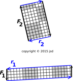
The torques r1∧F1 and r2∧F2 are calculated graphically in figure 34. By counting squares and considering the orientation, you can verify that the torques are equal-and-opposite. The diagram is not super-exactly to scale, but it’s pretty close; there are approximately 88 boxes in each diagram.
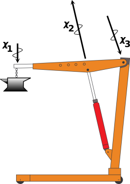
Everything in section 6.1 was kosher and above-board, but now we’re going to do something tricky. In the hands of an expert it is convenient, but in less-skilled hands it can lead to profound misconceptions.
In figure 35, the black arrows are doing double duty. The length and orientation of the χ1 arrow represents the force F1, while the location of the arrow represents the line of action of the forque.
A forque diagram such as figure 35 is sometimes called an interaction diagram. Sometimes it is called an “extended” free-body diagram (don’t ask me why). (It should not be called a force diagram.)
It must be emphasized that the arrows in figure 35 do not represent vectors. They are more than that. A vector has magnitude and direction, but not location, whereas the arrows in figure 35 have a partially-significant location. The location is significant insofar as the arrow must lie along the line of action, but the exact location is not significant insofar as you are free to slide the arrow parallel to itself along the line of action.
To say the same thing in different words:
| The length and orientation of the χ1 arrow represent a force, namely F1, the weight of the anvil. | The location of the χ1 arrow is being used to represent the line of action. |
Vehement suggestion: When in doubt, you should choose a datum and then draw each lever arm explicitly, as in figure 32. The lever arm is a vector with direction and magnitude, so you can represent it by drawing an arrow. Draw it and label it. Keep in mind that the force is a vector and the lever arm is a vector ... but they are not the same vector. Sometimes you can get away with using a single arrow to represent two vectors, but sometimes you can’t.
Again: By definition, a vector has a magnitude and a direction, but not a location. In diagrams, we normally use an arrow to represent a vector. However, in special situations, sometimes you can get away with using a single arrow to represent two vectors, or a vector and a bivector, or a vector and a projected point.
We are not changing the definition of vector, not under any circumstances. However, in figure 35 are tampering with the meaning of the arrows. We are using a single arrow to represent two things, a vector and something else. This is at best a sneaky trick, and sometimes it doesn’t work at all. The safest thing is to draw all the vectors explicitly, with one arrow per vector, as in figure 31 and figure 32.
Note the contrast:
| The black arrows in figure 35 have squiggles on them. That’s to indicate that they are more than vectors: they have a somewhat-significant location, not just magnitude and direction. They are located on the line of action. | If you were to leave off the squiggles, the diagram would become a trap for the unwary, because then you wouldn’t be able to tell whether an arrow was meant to represent a vector or something more. The arrows in figure 35 would become indistinguishable from the arrows in figure 31, even though the meaning is different. |
Here’s yet another reason why you should not become too enamored of diagrams such as figure 35: Although they are useful if you are interested in force and torque only, they are not satisfactory if you are interested in work and energy. Note the contrast:
| (10) |
where the subscript i is a reminder that there are typically multiple forces and multiple points of application, and you have to match them up properly.
You can use a single arrow to represent both Fi and ri∧Fi, but you can’t do the same for Fi and Fi·Δri. Therefore, as previously mentioned: The safest thing is to draw all the vectors explicitly, with one arrow per vector, as in figure 31 and figure 32.
We have two main ways of representing a forque. Here are some of the pros and cons:
| Force and Line of Action | Force and Torque |
| In simple situations, the idea of “line of action” works great and can provide useful insight. It is easy to diagram. | The idea of “Force and Torque” is not quite as intuitive, and not quite as easy to diagram. |
| It is elegant in the sense that it is gauge-invariant. You don’t need to pick a datum. | To quantify the torque, you generally need to pick a datum. Of course the observable physics is independent of the choice of datum; only the representation changes. |
| When the total force is zero, the choice of datum doesn’t matter. As a corollary, in a closed system, i.e. when there is no momentum flowing across the boundary, the choice of datum doesn’t matter. You can write the torque as a bivector, independent of any datum. |
| The idea of “line of action” doesn’t work particularly well in complicated situations, so you should not use it as the basis of your understanding. It is not convenient for calculations. Indeed, there are some forques that cannot be represented this way at all. | Once you pick a datum, the “force and torque” representation always works. It is convenient for calculations: To combine two forques, you just add the forces and add the torques. Every forque can be represented this way. |
| You can always rely on force and torque. You can always rely on momentum and angular momentum. | In simple situations, you may be able to get away with describing the forque in terms of force and line of action. |
| It is always safer and usually easier to keep track of the force and the torque. This makes the math very much simpler. | Trying to keep track of the force and the point of application is laborious and error-prone. |
| If you have a whole bunch of different forques, you can describe the overall situation by adding all the forces and adding all the torques. | If you have a whole bunch of forques, you cannot simply add the points of application. |
Note that if two bivectors have an edge in common, you can add the bivectors graphically, combining the areas edge-to-edge. We combine this with the fact that you can add vectors graphically, combining them tip-to-tail. This guarantees that the wedge product distributes over addition. For details on all this, see reference 12.
Also, from the definition of wedge product, it should be obvious that the wedge product of any vector with itself is zero. Combining this with the aforementioned distributive law, we obtain the following:
| (11) |
This is valid for any vectors A and F, and for any scalar c. It means that for any forque, we can shift the point of application and get exactly the same torque, provided we shift the point of application along a line parallel to the direction of the force. The geometrical representation of equation 11 is depicted in figure 36. The black arrows indicate shifting the point of application in a direction parallel to the force. High-school geometry tells us that the area of all such parallelograms are equal.
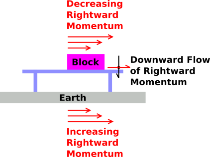
We now discuss momentum flow in another direction. Figure 37 is a snapshot of a block that is sliding to the right, sliding across a table that is fixed to the earth. There are no sideways forces on the block other than sliding friction. The block gradually decelerates due to friction.
| This means there is a downward flow of rightward momentum. That is to say, rightward momentum flows out of the block via the table into the earth. | Equivalently, we could say there is an upward flow of leftward momentum. Leftward momentum flows from the earth via the table into the block. |
Note that in this situation, the direction of momentum-transport (downward) is perpendicular to the type of momentum (rightward) that is being transported. A force of this type is called a shear force.
A shear cannot be classified as a push or a pull. Very roughly speaking, one might say:
In figure 37, note the symbol for shear. It consists of two parts: The red part indicates what is flowing, while the black part indicates the direction of flow. (This follows the same convention as used in section 3.1 to represent other types of momentum-flow.)
As mentioned in section 3.2.2, momentum-flow is not a vector. That means shear is not a vector. It is a symmetric second-rank tensor. If you rotate your point of view 180∘, the downward flow of rightward momentum would become the upward flow of leftward momentum ... which is exactly the same thing. (In contrast, if you rotate a vector 180∘ in any plane containing the vector, it would pick up a minus sign.)
Also
In figure 16, rightward momentum flows into train #1 via the red string.
In contrast, no energy flows through the string in this situation. The kinetic energy of the train is changing, so in accordance with the work/kinetic-energy theorem, there must be some mechanical work going on. Specifically, it takes energy to drive the winch that keeps the red string from going slack. We assume this comes from stored energy, stored within the train.
To repeat, there is a remarkable contrast: The momentum comes from outside the train, but the energy comes from inside the train. For details on this, see reference 13.
Both of these terms are problematic, because the names suggest that they are some special kind of vector, but but really they aren’t vectors at all. I insist that the point of application does not “belong” to the force, nor vice versa; both of them belong to the dynamic interaction, which is a higher-order abstraction.
| (12) |
When written that way, it’s obviously ridiculous ... but situations where the same word is used with two different yet deceptively similar meanings are exceedingly common. For example, a lap in the swimming pool is conceptually, qualitatively, and quantitatively different from a lap on the race track. Deceptive ambiguities are common even within physics: acceleration, heat, gravity, photon, charge, spin, etc.; see reference 6. It pays to be constantly on guard against such things.
Let’s be clear: Force is not a bound vector. Force is not a sliding vector. The arrows in figure 35 are not a one-to-one representation of the forces; each arrow represents a force and something else.
Here’s one way of knowing that force is not a bound vector: Consider the equation F=ma. The acceleration is not a bound vector, so therefore the force cannot be a bound vector. In physical terms: If I tell you the mass and the total force, you can calculate the acceleration of the center of mass ... but you have no idea where the point of application might be. So, again: the force that appears in F=ma is not a bound vector. It is not a sliding vector. It’s just a plain old vector, with direction and magnitude – nothing more, nothing less.
Here’s yet another way of seeing that a dynamic interaction is not really a vector. Consider the third law: for every force, there is an equal-and-opposite force. The point of application does not get negated! The counterpart interaction is an equal-and-opposite force at the same location. The force that is the subject of the third law is a plain old vector. The force gets negated.
In case you are wondering why I think in terms of momentum accumulating in a train car:
When I was seven or eight, we visited the Old Tucson movie studio. They had an old-time railroad car sitting there. For a joke, my kid brother and I posed as if we were pushing the railroad car, grunting and grimacing. Somebody said “that’s ridiculous” ... which we took as a challenge. So we spent the next several minutes pushing really hard. It turns out that railroad cars have very good bearings. If a couple of kids push for long enough, they can pour a huge amount of momentum into the thing. For several minutes, nobody paid any attention to us. Then my mother noticed what was happening and said “Hey, where are you going with that railroad car?”
This got our father’s attention, and he was appropriately horrified. By this time the car was moving right along. It wasn’t moving very fast, but it was definitely moving, and showing no signs of stopping.
We ran around to the other end and the two of us, plus our father, pushed on it in the opposite direction. It took a long time to get it stopped.