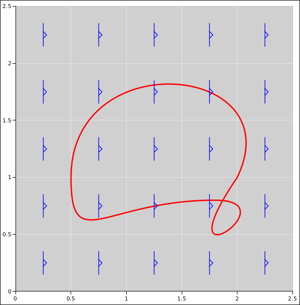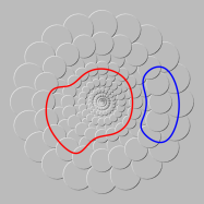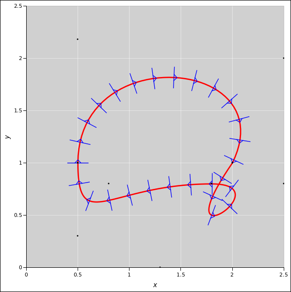
Figure 1: Arc Length around a Loop
Let’s start by considering Ferris Bueller’s car problem: Suppose you borrow a car, drive it around a complicated path, and then return it to exactly where you found it. Some things will return to their original state, but some will not:
| The X-coordinate (longitude) returns to its original value. The Y-coordinate (latitude) returns to its original value. | The distance traveled is nonzero. During the trip, the odometer reading advances by some nonzero amount. It does not return to its original value. |
A possible path is shown in figure 1. The total length of the loop is about 5.4 units. Along the path there are hash marks every 0.2 units.
We can understand this mathematically as follows: The element of arc length (ds) is defined via:
| (1) |
Now if we integrate around the loop, from start to finish, we find
| (2) |
The arc-length s is not a potential. There is no way you can join up the waymarks in figure 1 to create a well-behaved contour map. The s-value cannot be interpreted as a height.
Forsooth, if we consider the (x,y) plane to be our state space, s is not even a function of state. Now s is a perfectly good function of s as we move along the path, but s is not a function of location in the (x,y) plane. This is particularly obvious at the point where the path crosses itself.
The same goes for ds: We know the magnitude and direction of ds as a function of s as we go along the given path, but ds not a function of location in the (x,y) plane. This is particularly obvious at the point where the path crosses itself.
Let’s be clear: s and ds exist only in the low-dimensional space defined by the path. They are not functions of state in the higher-dimensional (x,y) state space.
The moral of the story is:
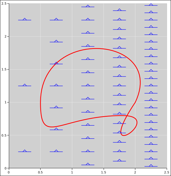
We can express x as a function of x and y. The gradient of this function is dx. Similarly, the gradient of the y-function is dy. These are shown in figure 2 and figure 3 respectively. The triangle on each waymark points uphill, in the direction of the gradient vector.
We see that dx and dy are very different from ds.
By definition, we say a vector field is grady if it is the gradient of some potential. Most vector fields are not grady, as discussed below.
An intermediate case is shown in figure 4. The waymarks represent the vector field 2x dy. This is intermediate in the sense that 2x dy is a perfectly good function of state in the (x,y) plane, so it is not as wacky as the element of arc length (ds) that we saw in figure 1. On the other hand, 2x dy is not the gradient of any potential, so understanding figure 4 is more work than understanding figure 2 or figure 3.
In figure 4 the waymarks are partially like the contour lines on a topo map, insofar as the closeness of the waymarks indicates the steepness of the local slope. On the other hand, there is no way you can join up the waymarks to make a well-behaved contour map. As you go from column to column, there are either too few or two many waymarks, so joining them is impossible. At every point, there is a notion of local slope, but the slope is not the gradient of any potential. A gradient can be integrated to find the height of the potential, but the slopes in figure 4 cannot be integrated to find a height in any consistent way, because the integral strongly depends on the choice of path. In particular:
| (3) |
In particular, if we integrate clockwise around the red path, we find that ∮cw x dy < 0, as can be seen in figure 4, as follows: when the path is going uphill (near the left side of the diagram) there are relatively few uphill waymarks, whereas when the path is going downhill (near the right side of the diagram), there are relatively more downhill waymarks.
The moral of the story is:
The diagrams in this section were created using the spreadsheet in reference 1.
In thermodynamics it is exceedingly common to encounter vector fields that behave like figure 4, i.e. things that are not the gradient of any potential. The poster child for this is T dS:
| Energy | | | E | | | scalar field | | | function of state | | | potential |
| Entropy | | | S | | | scalar field | | | function of state | | | potential |
| Temperature | | | T | | | scalar field | | | function of state | | | potential |
| | | dS | | | vector field | | | function of state | | | gradient of a potential | |
| | | T dS | | | vector field | | | function of state | | | not the gradient of any potential |
T dS is not grady (except in rare, trivial cases). There is nothing mysterious about this. Most fields aren’t grady. No explanation is required. Meanwhile, if you divide T dS by T, what remains is grady. There’s nothing mysterious about this, either. Obviously dS is the gradient of S.
For more about the application of one-forms to thermodynamics, see reference 2.
Here are some tangential remarks about things that are intriguing but far less important than they appear:
Some people call T dS the heat, by definition. However, that definition is not important for present purposes, and I am not interested in arguing about terminology. It suffices to let T dS go by the name T dS, pronounced “Tee dee Ess”.
The name “thermodynamics” means literally the dynamics of heat, so one might imagine that focusing on heat would be central to the study of thermodynamics, but it’s really not. Anything you can do in terms of heat and work can be done in terms of energy and entropy instead, with less effort and less ambiguity. For the details on this, see reference 3.
So the fact that T dS is neither a scalar nor the gradient of any potential turns out to be neither mysterious nor important.
Similarly, in electromagnetism, it is exceedingly common to encounter things like x dy − y dx, i.e. things that are not the gradient of any potential. In particular, sometimes people who ought to know better pretend that the voltage is a potential, even when it is not.
For more about the definition of voltage, including its dependence on the choice of path, see section 5 and reference 4.
In the real world, there are lots of things that locally have a notion of “uphill” and “downhill”, but don’t have a definite height. Examples abound in electromagnetism and in thermodynamics. Figure 5 may help you visualize what’s going on. In the figure, clockwise = locally downward, everywhere.
Non-experts tend to think that every force-field that is a function of position must be derived from some potential, but it’s just not true.
If you want a real-world example, imagine you are standing near a whirlwind. If you walk clockwise around the core of the whirlwind, the force of the wind is assisting you the whole way. If you walk counterclockwise, the force of the wind is opposing you the whole way. (Walk slowly, so that any dependence on your velocity is negligible.)
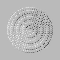
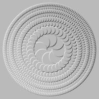
In the simplest case, a whirlwind can be described as a vortex, which has a particularly simple distribution of velocities, as shown in figure 6.
It is amusing to note that in an ideal vortex, if you care only about the velocity, the integral of velocity is the same along any simply-connected path that encompasses the core, such as the red path in figure 7. In particular, the integral is 20 steps, as you can verify by counting it yourself. Meanwhile, the integral is zero for any simply-connected path that does not encompass the center, such as the blue path in figure 7.
As another example, when talking about voltage, the recommended term is simply voltage. Beware that some people use the term “electric potential” as if it were synonymous with (or preferable to) the term “voltage”, but this is a horrible misnomer and misconception. There are innumerable cases where you have a voltage but you don’t have a potential. The notorious “ground loops” and other wiring loops are a case in point. If the voltage were a potential, you wouldn’t care whether your wiring had loops or not.
While ground loops are unhelpful, many helpful devices exploit the same physics, i.e. the fact that you can pick up a voltage by going around a closed loop. Examples include transformers, generators, and betatrons. As described in reference 5, a betatron uses a magnetic field that steadily increases as a function of time. For simplicity let’s consider a simplified betatron in which the magnetic field is spatially uniform, in which case the induced electric field is shown in figure 8.
In figure 8 you can see that the magnitude as well as the direction of the force is changing from place to place. In contrast, in figure 5 the magnitude is the same everywhere and only the direction is changing.
The electric field inside an ordinary transformer is definitely not the gradient of any potential. It is qualitatively similar to the betatron field.
(By the way: An unsuitable example would be the frictional force due to sliding on a stationary table-top. This force is not derived from any potential. It is a function of velocity, not a function of position. We aren’t discussing such forces here.)
In figure 5 or figure 8, pick two points A and B, and a definite path from one to the other. The height-change along the path is the number of upward steps you take going along the path, minus the number of downward steps. The answer depends on your choice of path, not just on the choice of endpoints. (For a potential, such as figure 10, the answer depends only on the endpoints, independent of path.)
If we want to get fancy, we can say each of these figures represents something called a one-form, as discussed in reference 6 and references therein. A one-form that is the gradient of some potential is called grady. A one-form that is not grady is called ungrady or non-grady.
Additional terminology: A grady force field is commonly called a conservative force field. Alas, this terminology is just begging to be misunderstood. In electrodynamics, for example, both grady and non-grady force fields uphold conservation of energy, conservation of momentum, conservation of charge, et cetera, so it seems very strange to call the non-grady fields “non-conservative”.Also: Many books refer to a grady one-form as an exact differential, and an ungrady one-form as an inexact differential. Alas, this terminology is also begging to be misunderstood. Beware that in this context, inexact does not mean imprecise or approximate. Not at all. Also beware that an inexact differential is really not a differential at all.
To summarize:
| (4) | ||||||||||||||||
Compared to the concept of “inexact differential”, the concept of ungrady one-form is more modern, more powerful, and easier to visualize.
To be explicit: The force at each point in the field depicted by figure 5 has components given by:
| (5) |
In this case the magnitude of F is constant everywhere, and F points clockwise everywhere.
The corresponding equations for the non-conservative force acting on the electron in the betatron are actually simpler, even though figure 8 appears more complicated:
| (6) |
In this case, the magnitude of F is proportional to the radius. Again, F points clockwise everywhere. This field has the interesting property that it has the came amount of curl everywhere. That is, if you go clockwise around a closed loop anywhere in the betatron electric field (figure 8), the net number of downward steps that you take is proportional to the area of the loop, independent of the shape of the loop. Try it.
You can easily verify that neither of these force-fields can be the gradient of any potential. (Hint: d ∧ d Φ = 0 for any potential Φ. If you insist on writing this hint in terms of cross products, which I don’t recommend, the expression is ∇ × ∇ Φ = 0.)
A more aesthetic non-potential is presented in figure 9 but it isn’t quite as precise or generalizable.
Let’s discuss the technique used to represent one-forms in figures such as figure 8. I call this the fish-scale representation.
These fish-scale diagrams are a big help, because they are a convenient way to portray ungrady one-forms.
When talking about the forces and about the energy, we must be careful to keep track of which is which.
I don’t consider this technique an optical illusion. I consider it a non-deceptive way of portraying one-forms such as the electric field in a betatron.
The portrayal has various minor imperfections, including:
Also we must be careful when using the word "downward" (as in "clockwise = locally downward everywhere").
The boundary of a scale is meaningful. The question of whether one scale is above another scale is not meaningful.
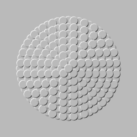
The fish-scale representation works fine for grady as well as ungrady one-forms. Figure 10 shows something that is a potential, namely a conical bump. The bump has a slope, which is a grady one-form.
Other representations are sometimes possible. Much depends on whether the state has a metric (i.e. a dot product). Consider the contrast:
| Metric | No Metric |
| In many situations, do have a metric. Ordinary position-space is a good example. Rectangular (Cartesian) coordinates can be used to induce a nice, simple, familiar metric. You can also use polar coordinates (in 2D or 3D), but the induced metric has singularities and other complications, and must be used with care. Also, in special relativity, spacetime has a metric, although it is slightly peculiar. And so on. | On the other hand, there some situations where we lack a metric. Thermodynamics is an exceedingly important example; see reference 2. There are also situations, such as general relativity, where the metric might be unknown, or so complicated that we don’t want to deal with it. |
| In such situations: The metric defines for us a notion of length and a notion of angles. We can use that to create a dual representation where every one-form corresponds to a vector and vice versa. A vector field can be represented by placing, at selected points, an arrow representing the magnitude and direction of the vector at that point. Usually the length of the arrow is used to encode the magnitude of the vector, but sometimes barbs are used instead, as discussed in reference 7. | In such situations: Without a metric, there is no way to associate a one-form with a “corresponding” vector, nor vice versa. One-forms are not readily representable in terms of arrows. This makes the fish-scale representation particularly valuable. |
The fish-scale technique can be considered a modification of conventional mapmakers’ techniques for depicting relief, including contour lines, shading, et cetera.
On a map drawn in two dimensions, the contours are contour lines. In three dimensions the contours are surfaces, also called shells. More generally, in a space of dimension D, the contours are hypersurfaces of dimension D−1. We note in passing that the fish-scale technique can be generalized to higher dimensions. In the D=2 fish-scale diagrams, you see lots of 3/4-complete circles. In D=3, the corresponding elements will be 3/4-complete spheres, each nestled against its neighbors. The techniques of shading to portray the orientation of the contour also generalizes. For now, though, we will concentrate on the two-dimensional case.
Plain old contour lines are problematic even for grady one-forms. For one thing, they don’t “grab” the viewer. A related problem is that contour lines don’t distinguish an upslope from a downslope. You can’t tell a pit from a peak. When cartographers want to create a map with visually perceptible relief, they must supplement (or replace) contour lines with various shading and/or color-coding schemes.
For ungrady one-forms, contours are even more problematic.
People often speak of contours as equipotentials, although technically you can’t have equipotentials if you don’t have a potential. Still, you can have the next best thing, namely constant-energy contours. Start at an arbitrary point. Shoot out “trial move” vectors in every direction. Make a note of the directions in which the trial move causes zero change in energy. Move a small distance in that direction, and iterate. This maps out the constant-energy contour. As long as you stay on this contour, your energy doesn’t change. (One thing you cannot do is label this contour as to energy, because if you leave the contour and come back to it, you will in general have a different energy.)
These constant-energy contours do a good job of portraying the orientation of a one-form even for an ungrady one-form (i.e. a non-conservative force field). However, portraying the orientation is only half the battle. Recall that we have multiple objectives:
With grady one-forms, both objectives can be achieved with high accuracy. You choose contour lines that are evenly spaced in energy.
With ungrady one-forms, there is a terrible dilemma. Suppose you map out the constant-energy contours using the method described above. When you attempt to represent the magnitude of the one-form, you will find that if the spacing between contours is correct in one region it will be incorrect in neighboring regions. You will have to start new contours here and there. There is no way to do it perfectly.
Just to rub salt in the wound, the shading techniques that work for a grady one-form look hideous when applied to the discontinuous contour lines that are characteristic of an ungrady one-form.