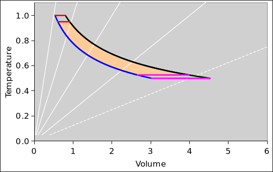
Figure 1: Engine, Driven Hard
Let’s see if we can understand how the efficiency of an ordinary engine varies as a function of how hard we drive the engine.
We imagine that the engine is operating at constant cycle-time, i.e. constant rotational rate, so the amount of power output is proportional to the torque. For details on how this might be arranged, see section 1.3.
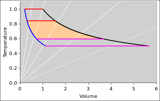
Figure 1 shows some (but not all) of what happens when the engine is driven hard. The inner yellow-shaded region tells us roughly how much useful energy the engine puts out per cycle. (If this were a PV diagram instead of a TV diagram, the area would be exactly the energy.) The outer unshaded loop shows what the engine would do if there were no losses of the kind considered in reference 1, i.e. no series dissipation.
The white lines in these diagrams are contours of constant pressure. They are not particularly important for the current discussion. They stand in contrast to the contours of constant V (which are vertical) and the contours of constant T (which are horizontal). The contours of constant entropy are curves, trending roughly from the upper left to the lower right; the blue and black curves are examples.
In operation, the engine moves clockwise around the path shown in these figures. The red and black portions involve expansion of the working fluid, while the magenta and blue portions involve compression.
Figure 2 shows some of what happens when the engine is driven less hard. Remember, this is a constant-speed engine. Because we are transferring less entropy – or, loosely speaking, less “heat” – into the engine per cycle, the series temperature drop is less. Therefore the unshaded areas at the top and bottom of the cycle are smaller in the dT-direction. They are also smaller in the dV direction, just because the whole cycle is smaller in that direction. Putting the two factors together, we see that the series dissipation depends more-or-less quadratically on how hard we drive the engine.
Beware that these diagrams show only the series dissipation, not the parallel losses. The importance of this will be discussed in section 1.2.
The spreadsheet for making these Carnot plots is cited in reference 2.
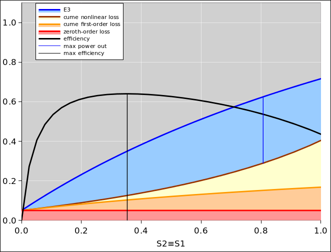
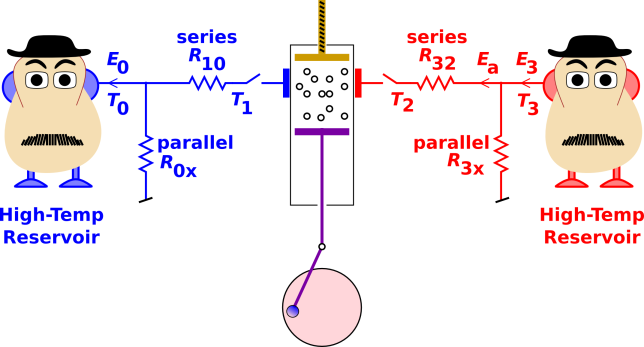
In figure 3, the horizontal axis represents how hard we are driving the engine. We quantify the drive in terms of S2, the entropy the flows through the subengine.
Terminology: In the spreadsheet (reference 3) and in this document, the term “subengine” refers to the inner engine that operates reversibly between temperatures T2 and T1 ... in contrast to the overall engine that operates irreversibly between temperatures T3 and T0. The overall engine is irreversible because of the parallel losses and series dissipation. The definition of E3, T2, et cetera can be inferred from figure 6.
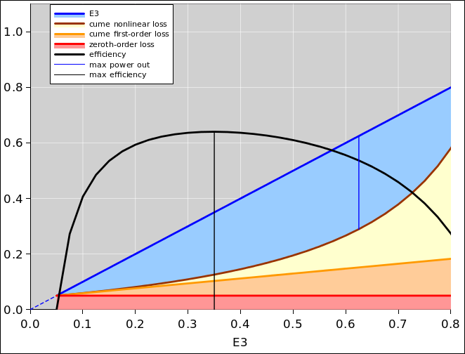
Since E3 is a nice monotonic one-to-one function of S2, we can replot the data using E3 as the abscissa. This is shown in figure 4. Note that E3 is the total energy used by the overall system. Figure 3 has the advantage of more closely reflecting the details of the model, while figure 4 makes some of the final results easier to interpret.
In both figures:
A frictional force proportional the square of velocity would make a contribution to the power that is third-order in the velocity. This would apply to fluids at high Reynolds number. I’m not sure how relevant this is to typical engines. This would require a new band to represent the third-order contributions.
Note the contrast: The zeroth-order term represents thermal losses in parallel, while the second-order term represents series dissipation.
The model we have just set forth can be described via an equation:
| (1) |
where S1 is equal to S2 and represents the entropy flowing through the subengine. The RHS of this equation is considered a function of S2. It is nonlinear, because T2 and T1 are functions of S2. This stands in contrast to T3 and T0, which are considered fixed, independent of S2.
We can expand the RHS in a Taylor series. This gives us a phenomenological two-parameter model:
| (2) |
The energy here represents the energy per cycle. Ditto for the entropy. Because this engine is running at a constant rate, the distinction between power and energy per cycle is not very important. As a related point, the “time” variable does not appear in equation 1 or in the spreadsheet in reference 3.
The constant-rate simplification does not result in any loss of generality. You could perfectly well run the model engine at constant torque and variable rate. There would still be zeroth-order, first-order, and second-order losses. The calculations would follow the same pattern and the conclusions would be the same. There would be a slight change in terminology, but that’s all.
Normally a second-order polynomial is a three-parameter model, but in equation 2 there are only two adjustable parameters. That’s because the coefficient of the linear term is determined for us in terms of the specified parameters T3 and T0, determined by conservation of energy in the limit of small S2.
In the legend of figure 3, the word “cume” stands for cumulative. It reminds us that the brown line at the top of the nonlinear band represents the cumulative losses, including zeroth-order, first-order, and nonlinear losses (not just nonlinear).
| (3) |
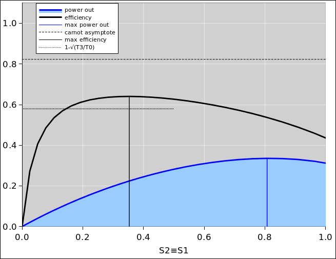
and is independent of how hard we drive the engine. In the example shown in figure 3 and figure 5, the Carnot efficiency is just over 0.8. This is shown in figure 5 by the horizontal dashed black line.
This Carnot efficiency could be obtained by using a high-side temperature of T3 = 1400 C and a low-side temperature of 27 C, which are reasonable numbers for a real-world power plant. However, in the spreadsheet in reference 3, we normalize the temperatures so that T3 = 1. In normalized units, our example uses β = 0.05 and γ = 1.0.
Figure 5 shows the same situation. The power out curve is shown by itself, riding on a zero baseline, rather than riding on top of the cumulative losses. This makes it easier to recognize the max-power point as being the max-power point.
Let’s do a little bit of engineering analysis. Let’s suppose, temporarily and hypothetically, that we start out operating at the max-power point, at about 0.85 on the “S1” axis as shown in the figure. Nobody in his right mind would continue to operate at this point. That’s because throttling back a little saves fuel to first order, but leaves the power output unchanged to first order. If we throttle back all the way to 0.6, there is only a tiny decrease in power, but there is a substantial increase in efficiency ... as you can see by comparing the blue and black curves in the figure.
Because nobody ever operates near the max-power point, engines are not even designed to permit that. The redline operating limit of the engine will be set much lower, so that the internal parts do not need to be nearly as strong.
The peak efficiency comes out to be approximately 1−√(T0/T3), as shown by the short horizontal dotted line. This is a coincidence, devoid of any deep physical meaning.
The power produced at the drive shaft of any engine is given by the rotational rate multiplied by the torque.
We now restrict attention to the special case where the rotational rate is constant. This simplifies the math. It is not unduly unrealistic, because:
We can build a simplified pedagogical model of an engine that works this way by slightly modifying the usual Carnot-type engine. The key modification is to provide for an adjustable compression ratio. The general idea is shown in figure 6.
We can adjust the compression ratio by moving the cylinder head, shown in tan, at the top of the cylinder. Any such adjustment happens very slowly relative to the cycle time of the engine.
The compression ratio in figure 1 is about 12.05, while the compression ratio in figure 2 is about 6.57. You can read the graphs to get the max volume (at the black/magenta corner) and the min volume (at the blue/red corner) and take the ratio.
As previously mentioned, the red and black parts of the path involve expansion of the working fluid, while the magenta and blue parts involve compression. There is some timing involved. That is, we need to engineer the engine so that the proper fraction of the expansion is isothermal and the proper fraction is isentropic. Ditto for the contraction. The mechanism for doing this is not shown in figure 6. The timing changes quite a bit, depending on how hard we are driving the engine.
The spreadsheet (reference 3) needs to calculate the temperature at the low side of the subengine. This involves solving two simultaneous equations
| (4) |
| (5) |
Plugging one into the other we find
| (6) |
Also note: in the spreadsheet, the resistor from T0 to ground is ignored. All of the parallel losses are attributed to the resistor from T3 to ground.
The inverse of efficiency is specific fuel consumption. Efficiency is elegant, and is usually expressed in dimensionless units. Specific fuel consumption is practical, and is usually expressed in practical units, such as pounds of fuel per horsepower-hour.
In a real power plant, vehicle, or aircraft, there are various places to measure the power. In an electric power plant, we could measure the mechanical power at the output shaft of the prime mover, or we could measure the electrical power at the output of the dynamo.
The term Brake Specific Fuel Consumption (BSFC) refers to mechanical power at the output shaft, as measured by a device known as a prony brake.
Let’s consider the energy budget of a car engine when it is idling in neutral. The output shaft is delivering zero power, yet the fuel consumption is nonzero. Therefore the BSFC is infinite. The efficiency is zero. At any speed less than the idle speed, we are faced with some difficult concepts, because in some sense the BSFC is “more than infinite” and the efficiency is “less than zero”.
Reference 1 sets forth an oversimplified one-parameter model and compares it to “some” power-plant data. It checks the predicted efficiency against observed efficiency. Alas, this is not a very incisive check.
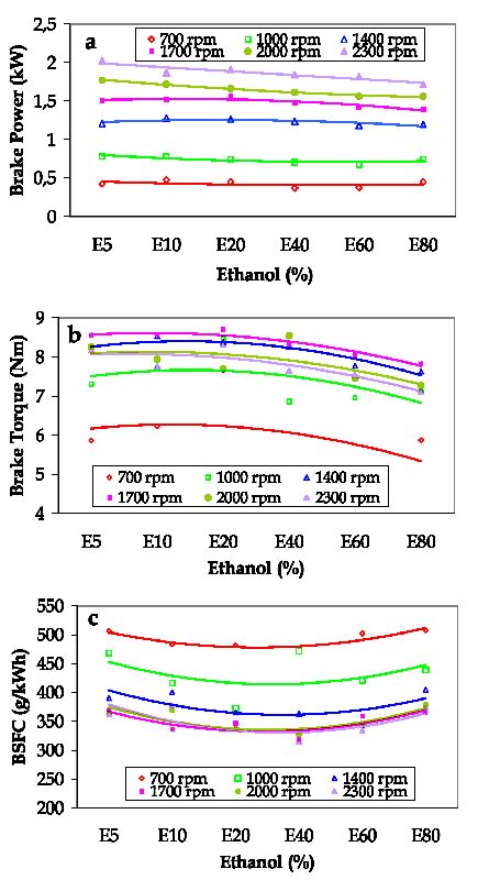
It is vastly better to check the BSFC as a function of operating speed. Figure 7 shows the data for a Waukesha VGF F18, which is a stationary natural-gas-fired 6-cylinder engine, used for electrical power generation. It is rated for 400 hp at 1800 RPM. The data is from reference 5. In the figure, the various colored curves correspond to various experimental lubricants.
The data in figure 7 shows that for this engine, normal operation is actually slower than the max-efficiency point. It is far, far slower than the max-power point. Also, it completely disproves one of the central claims made by reference 1, namely that the engine should become more efficient at lower speeds. I’ve seen lots of BSFC maps, and in every case I can think of, the BSFC gets worse (not better) as the speed goes down, in the lower part of the operating range.
Logic suggests that the Curzon/Ahlborn argument should apply even more strongly to trucks and aircraft, where one is interested not only in power, but also in power-to-weight ratio. There is considerable incentive to install an undersized engine and run it extra-hard, even if this entails some loss in thermodynamic efficiency.
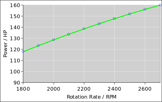
However, the Curzon/Ahlborn argument fails miserably when applied to real-world aircraft engines. Figure 8 shows the power versus rotation rate for a Lycoming O-320 engine, a widely-used aircraft engine. The circles are taken directly from the O-320 Operator’s Manual. The green line comes from a numerical model of engine performance, as used in a flight simulator.
The manual specifies that redline is 2700 RPM. That is to say, the engine is never operated at any higher rotation rate. This is marked by – you guessed it – a red radial line on the tachometer.
Typical cruising flight is conducted at 2400 RPM or thereabouts, depending slightly on altitude.
It should be obvious from the figure that power is an increasing function of rate, throughout the permissible operating range. This engine is never operated at the max-power point. Not even close.
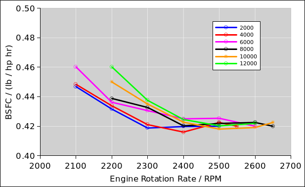
The BSFC is a declining function of rate throughout the permissible operating range, as shown in figure 9. The corresponding efficiency (not plotted) is an increasing function of rate. The various colored curves correspond to various operating altitudes.
Operating the engine at higher rates would be be less efficient ... especially if we factor in the propeller, i.e. if we think in terms of effective thrust power (not just brake power), as we should. In response, the engine components were designed with only enough strength to handle redline speeds, where redline is far below the max-power point. Designing the engine to operate at the max-power point would have made it heavier and more expensive, for no good reason.
The data in figure 9 shows that for this engine, normal operations are conducted near maximum efficiency. Also, it completely disproves – again – one of the central claims made by reference 1, namely that the engine should become more efficient at lower speeds.
Figure 10 shows more of the same. The data is from reference 6. The normal operating point is near max efficiency. It is nowhere near max power. The BSFC gets worse, not better, at the lowest throttle settings.
Airline companies care a great deal about fuel efficiency. They sometimes decommission perfectly serviceable airliners and buy new ones – at $200,000,000.00 apiece – in order to get improved fuel economy. See reference 7.
Let’s compare the two-parameter model presented here to the one-parameter model presented in reference 1 and elaborated in reference 4.
| jsd two- | C/A one- | |||
| parameter | parameter | |||
| model | model | |||
| Operating point is at or | no | yes | ||
| near the max-power point. | ||||
| Operating point is at or | yes | no | ||
| near the max-efficiency point. | ||||
| Efficiency at operating point | yes | yes | ||
| is on the order of 50% of | ||||
| the Carnot efficiency. | ||||
| Driving the engine less hard | decrease | increase | ||
| would cause the efficiency to: | ||||
| At zero drive, the efficiency is | less than zero | at a maximum | ||
| Zeroth-order losses are | yes | no | ||
| essential to understanding | ||||
| the concepts and principles. |
The two models disagree on five out of the six predictions... and even the one point of agreement is largely illusory. The operating points are wildly different because the abscissas are different, so the fact that the ordinates are similar means little, if anything. In other words: I consider the agreement as to efficiency at the operating point to be fortuitous and devoid of real significance.
Not only are the conclusions of the C/A model grossly wrong, even the premises of the model are absurd. The model is predicated on the assertion that efficiency doesn’t matter. This assertion is exceedingly implausible, and is supported by precisely zero evidence.
The model in reference 1 is sometimes summarized by saying
which is a wrong explanation in support of an absurd conclusion.