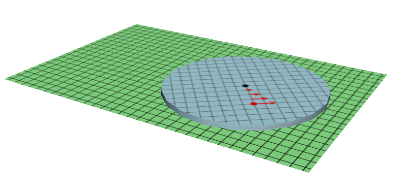
Figure 1: Rotating and Non-Rotating Coordinate Systems
At the park near my house, there is a small merry-go-round. A cartoon of the situation is shown in figure 1.
1) The merry-go-round is rotating. We imagine a reference frame attached to the merry-go-round, as indicated by the circular light-blue area.
2) We also imagine a non-rotating reference frame, as indicated by the rectangular green area. Loosely speaking, we imagine this reference frame to be attached to the ground. That is, we ignore the fact that the earth is slowly rotating. This is OK because the earth’s rotation is very slow compared to the rotation of the merry-go-round, in the situations of interest.
The following is common knowledge among the children in the neighborhood: Suppose you are riding the merry-go-round, sitting somewhere not too near the pivot, analyzing things relative to the rotating frame. You set a baseball on the floor of the merry-go-round and hold it stationary relative to the rotating frame for a moment. When you let go, the ball does not remain stationary; it accelerates outward. The initial acceleration is directly outward, radially away from the pivot.
The technical name for this is centrifugal acceleration. Please don’t tell me there is no such thing as centrifugal acceleration. It is a readily-observable physical fact. It is characteristic of rotating reference frames.
The magnitude and direction of the centrifugal acceleration varies from place to place in the rotating frame. Therefore we call it the centrifugal field. It is zero at the pivot. The farther we go from the pivot, the stronger it gets. It is everywhere directed radially outwards from the pivot.
It must be emphasized that the centrifugal field is associated with the rotation of the reference frame. It exists in rotating frames and not otherwise. In particular when describing the motion of the baseball relative to the non-rotating reference frame, we can (and should) explain everything we see without any contribution from the centrifugal field.
s The centrifugal field is not necessarily associated with the rotation of any material object. (A reference frame is something of an abstraction, and we can have a reference frame that is not tied to any material object.)
According to Einstein’s principle of equivalence, at each point in space, the gravitational field is indistinguishable from an acceleration of the reference frame. Einstein explained this in terms of the famous “elevator” argument. Please don’t try to tell me that Einstein’s argument is valid for elevators but not valid for merry-go-rounds; it’s the same physics in both cases. We conclude from this that the centrifugal field is as real as the gravitational field. Forsooth, at each point, the centrifugal field is indistinguishable from the gravitational field.
Both the gravitational field and the centrifugal field can be made to vanish, locally, by choosing a suitable reference frame.
As we shall see in section 1.2 and quantify in section 2, the equations of motion in the rotating frame contain additional terms, notably the Coriolis term (not just the centrifugal term).
| In an introductory physics class, the teacher might decide that a formal analysis of rotating frames is “beyond the scope of the course”. That’s OK with me. Actually I recommend going one small step farther than that, and explaining that centrifugal field exists in a rotating frame and not otherwise. That allows the students to see the boundary between what they can handle and what they can’t. | It would be completely unreasonable to say that rotating frames do not exist or that the centrifugal field does not exist. The physics of rotating frames has been understood for more than 180 years. |
It must be emphasized that everybody, in physics class and elsewhere, uses rotating frames routinely. In particular, the usual “laboratory frame” is a rotating reference frame, co-rotating with the earth. If you measure the magnitude and direction of the gravitational acceleration g, the result is different from what it would be in a nearby non-rotating frame. It’s only a small percentage difference, but it’s huuuuge compared to the precision of the measurement, even using high-school grade equipment and procedures.
There is no need to formally analyze the rotation of the lab frame. Just patch it up by fudging the direction and magnitude of g, and leave it at that. It is still possible to observe the rotation, using e.g. a Foucault pendulum or a decent gyroscope, but the introductory class mostly refrains from measuring things (other than g) that are sensitive to the rotation.
It is purely a matter of interpretation whether we should say the centrifugal acceleration corresponds to a centrifugal force, or whether we should call it an unforced acceleration. De gustibus non disputandum. That is to say, there is no point in debating the matter, because the equation of motion is the same no matter which way we interpret this point. See reference 1 for details on this.
If somebody asks about centrifugal force, it is usually best to answer in terms of centrifugal field and centrifugal acceleration. If the answer cannot be expressed in those terms, there is probably something wrong with the question.
The tricky question of how and why you feel the effects of gravity is discussed in reference 2.
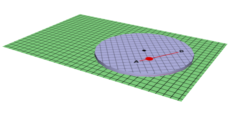
We can get a qualitative appreciation for the physics involved in the Coriolis effect by considering the situation shown in figure 2. We have a puck (shown in red) that is initially at rest in the rotating reference frame. It is held in place by a string (not shown) running from the pivot to the puck. The string serves to counter the centrifugal force.
We now consider what happens when we pull on the string, pulling the puck toward the pivot. By conservation of angular momentum, the puck’s velocity must increase, in inverse proportion to its distance from the pivot. These velocity vectors are shown in red in figure 2. Note that these are velocity vectors as measured in the nonrotating frame! As a reminder of this point, look at the initial velocity vector, which would be zero in the rotating frame, since the puck is initially at rest in the rotating frame.
Now let us consider a slightly different scenario, the scenario we really care about, where the puck is guided by a rail in the rotating frame, so that when we pull it toward the pivot it must move directly toward the pivot.
The velocity that the puck must have at each point as it moves along the rail is shown in figure 3. The velocity varies in direct proportion to the distance from the pivot, which is the familiar rule for the rotation of a rigid body such as our merry-go-round.
The rail must exert a force on the puck to keep it moving directly toward the pivot. There are two terms that contribute to this force (plus a centrifugal force that we are ignoring for the moment).
Each of the two Coriolis terms is a product, proportional to how fast the frame is rotating multiplied by how fast the particle is moving relative to the rotating frame (i.e. how fast we pull on the string).
In the non-rotating frame, this force requires no special explanation; it is just the force required to make the puck follow a non-straight path as it spirals inward. In contrast, in the rotating frame, the puck is following a straight path, and we wish to preserve the spirit of the first law of motion, namely that a particle should move in a straight line if and only if it is subjected to no net force.1 So we say that there is a Coriolis force (to the right in this case) and the mechanical force exerted by the rail serves to counter the Coriolis force.
Beware that it is extremely common to find wrong explanations of the Coriolis effect. Most of the hand-wavy explanations are off by a factor of two. In effect they blow off the factor of 2 in front of the Coriolis term in equation 12 and all similar equations.
We can guess where this mistake comes from by comparing figure 2 with figure 3. The former says that as the puck is pulled inwards, the velocity “would” increase if the puck were not constrained by the rail, while the latter says that the velocity “should” decrease if it is to match the rigid-body rotation. So there are two contributions to the physics ... and they turn out to be numerically equal. Anybody who notices half the physics but overlooks the other half will get the wrong answer by a factor of 2.
Another moderately common mistake is to suggest that the force exerted by the rail is the Coriolis force. This is backwards. In our scenario the Coriolis force pushes to the right; the rail counters the Coriolis force by pushing to the left. The Coriolis effect exists whenever an object is moving relative to the rotating frame (whether or not it is opposed by a rail or anything else).
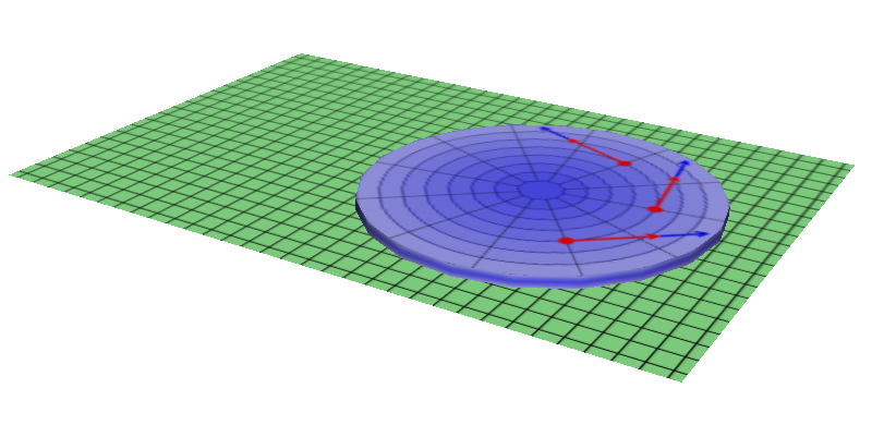
Let us now try to get a qualitative understanding of the Coriolis effect in the case where the puck is moving tangentially, as shown in figure 4. As before, the puck is shown in red, and the velocity vectors are measured in the nonrotating frame. A string holds the puck at a constant distance from the pivot. The puck is moving relative to the rotating frame, swinging like a tetherball, moving in the locally tangential direction.
- Relative to the rotating frame, at each point, the velocity of the puck is given by the blue vector in the diagram.
- Relative to the nonrotating frame, the velocity of the puck is given by the sum of the red vector and the blue vector. The red vector accounts for the rotation of the frame itself.
The figure shows three snapshots of the puck at three successive times. As the puck moves from place to place relative to the rotating frame, not only does its position change, but its velocity changes also. The string must apply a leftward force to the puck to impart a change in momentum, to turn the velocity vector to the left. Some of the tension in the string is needed to oppose the centrifugal force – which is independent of the blue velocity – but there is another contribution which is proportional to the blue velocity, which is needed to oppose the Coriolis force.
When we analyze the situation in the nonrotating frame, we again find two Coriolis terms (plus a centrifugal term), each of which is a product:
To summarize this section: Suppose the rotating frame is rotating counterclockwise. We have an observer moving relative to the rotating frame, facing forward along the direction of motion. We have shown that there will be a Coriolis force directed to the observer’s right. We have explained this in the case of northward motion and in the case of eastward motion. From there it is only a small leap to hypothesize a similar effect for all other directions of motion.
If you do the math – as in section 2 – you discover that in all generality, whenever an object has a velocity relative to some rotating frame, the Coriolis force is perpendicular to that velocity. You can find the direction of the Coriolis force by projecting the velocity onto the plane of rotation, then rotating the projection 90 degrees counter to the rotation of the frame.
We now start building a quantitative understanding of motion in a rotating frame. The set of equations of motion we use in such a frame is different from the set of equations we would use in a non-rotating frame. The two sets of equations are consistent with each other, and indeed each can be derived from the other, as we now demonstrate.
For additional details about the laws of motion, see reference 3.
Suppose we have a pointlike object whose position is described by the abstract vector Q. This vector has components Q@J relative to the nonrotating laboratory frame, and components Q@M relative to the rotating frame.
Let’s see if we can express Q@M in terms of Q@J (and in terms of the other “givens”). We can get a good start just by turning the crank.
Let’s start with plain old position. To connect the position in one frame with the position in the other frame, we write
| Q@J = R{θ}(Q@M) (1) |
where R{θ}(⋯) is the rotation operator that rotates something by an angle θ in our chosen plane of rotation.
We need to operate on this rotation operator. This includes being able to differentiate with respect to θ. This is easy to do if we know how to multiply vectors, as briefly defined in section 5.3 and more fully explained in reference 4. That allows us to express the rotation operator in terms of rotors, as briefly defined in section 5.4 and more fully explained in reference 5. Using that representation, we have:
| (2) |
where γ1 and γ2 are any two orthonormal vectors in the plane of rotation, and θ is the angle of rotation of the rotating frame relative to the laboratory frame, and r() is a rotor that generates a rotation in this plane, as discussed in section 5.4.
Now we can calculate the velocity, based on the position we just calculated. To do that, we differentiate both sides of equation 1. For simplicity we assume the plane of rotation is unchanging.
| (3) |
where the “dot” denotes differentiation with respect to time.
This can be put into a nicer form if we factor out γ1 γ2 in a couple of places:
| (4) |
The first two terms on the RHS of equation 4 look tantalizingly similar, and indeed using
equation 21 we can combine them to yield:
| (5) |
where ρ is defined to be the projection of Q onto the plane of rotation. This definition is valid in any frame (M or otherwise). That is:
| ρ := (Q − γ2 γ1 Q γ1 γ2) / 2 (6) |
Equation 5 can be made slightly more symmetric-looking by use
of equation 24:
| (7) |
Or, switching back to the more condensed “rotation operator” notation,
| (8) |
The second term on the RHS of equation 8 can be interpreted as a rotated version of the “ordinary” velocity, namely the time-derivative of position, in close analogy to the LHS of the equation. Meanwhile, the first term on the RHS is an additional contribution, a “tangential velocity” term due solely to the rotation of the frame. It exists whether or not the object is moving relative to the rotating frame. It lies in the plane of rotation, and is 90 degrees “ahead” of the radial position vector ρ@M.
Let’s continue to turn the crank. To form the second derivative, we differentiate both sides of equation 7.
| (9) |
which can be simplified by collecting like terms, i.e. combining the 2nd and 3rd lines, and combining the 5th and 6th lines:
| (10) |
and that can be further simplified by some simple algebra:
| (11) |
and put into more compact form:
| (12) |
where we have introduced ω := θ• to denote the rate of rotation.
The interpretation of the various terms on the RHS of equation 12 will be discussed in a moment, in connection with equation 14, but we can already begin to see what’s going to happen: The last term is a duly rotated version of the “ordinary” acceleration. The third term is destined to give rise to the Coriolis effect. The second term is destined to give rise to the centrifugal effect. The first term accounts for changes in the rotation rate.
The terms pre-centrifugal and pre-Coriolis bear the prefix “pre-” because we need to uphold the principle that the centrifugal field and the Coriolis effect exist in the rotating frame and not otherwise. Since equation 12 is nominally an expression for the acceleration in the nonrotating frame, as specified by its LHS, these are not really centrifugal or Coriolis terms. They don’t even have the correct signs. We will obtain the final correct expression (equation 14) in a moment.
Equation 12 has the elegant property of having the Q@J-related term on one side, and all the Q@M-related terms on the other side. This makes clear the role of these equations; they are simply the mapping from one coordinate system to another.
We now sacrifice elegance by rearranging the equation to isolate Q@M•• on one side:
| (13) |
or, in more compact notation:
| (14) |
So, finally, we have an expression for the acceleration in the
rotating frame.
| The last term on the RHS is a duly rotated version of the “ordinary” acceleration, i.e. the second derivative of the position, in close analogy to the LHS of the equation. | It is independent of position and independent of velocity. |
| The third term describes the Coriolis effect. | It is proportional to ρ@M• (the velocity in the rotating frame, projected onto the plane of the rotation) and also proportional to ω (the rate of rotation of the frame). This term is independent of position. It lies in the plane of rotation, and is perpendicular to the velocity. |
| The second term describes the centrifugal field. | It is proportional to the square of the rotation rate, and also proportional to ρ@M (the distance from the axis of rotation). It is independent of velocity. |
| The first term describes the effect of unsteady rotation. Any observer attached to the rotating frame will be “swatted” as the rotation rate increases or decreases. | It is proportional to the distance from the axis of rotation, and proportional to the rate of change of the rotation rate of the frame. It does not depend on the puck’s velocity relative to the rotating frame (unlike the Coriolis effect). It vanishes in the case of steady rotation. It is often neglected. |
Remark: The word “centrifugal” means, literally, fleeing away from the center. The rearrangement leading to equation 14 changed the sign of the ω2 ρ@M term, so that now it more clearly deserves the name “centrifugal”, in the sense that the centrifugal term ω2 ρ@M is directed radially outward, making an outward contribution to the acceleration Q@M••. Similarly the Coriolis term in equation 14 has the correct sign. Since −R{90∘}(⋯) = R{−90∘}(⋯), we can say that the Coriolis force is 90 degrees behind the velocity vector, where the notions of “ahead” and “behind” are defined by the direction of rotation of the rotating frame.
Note that ρ@M is directed radially outward, by definition, by construction.
There are various possible reasons why you might want to use equation 14. For example, suppose you already know Q@J•• somehow, and you wish to solve for Q@M by timestepping the equation of motion. Equation 14 will tell you the current value of Q@M••, which you can integrate to get the next value of Q@M•, and so forth.
In particular, we might know Q@J•• from the second law of motion, equation 17. In its usual form, this law is not valid in rotating frames, but for present purposes that’s no problem. We simply apply the law in the nonrotating frame. This gives us the acceleration-components Q@J•• in terms of the force-components FJ.
Plugging in, we immediately obtain:
| (15) |
At this point we have the option of applying the distributive rule in
reverse to pull a factor of (1/m) out of every term on the RHS.
Doing so means that each of the terms within braces now has dimensions
of force:
| (16) |
Here’s an amusing mnemonic: If we restrict attention to uniform rotation, so that the swat term vanishes, the remaining three terms on the RHS of equation 14 has the same structure as a binomial expansion, namely (a+b)2, namely a2 + 2ab + b2. In this case a is the frequency omega, while b is, roughly speaking, the time derivative operator, denoted by a dot in the equations. The centrifugal term has two copies of ω, the ordinary F=ma term has two copies of the time derivative, and the cross term, i.e. the Coriolis term, has one copy of omega, one copy of the derivative, and a factor of two out front. Don’t forget the factor of two.
Equation 12 and equation 14 are not the almost general expressions, because we have assumed that the plane of rotation is not varying. In a two-dimensional world, this is obviously OK, but in three dimensions it is perfectly possible to be rotating around an axis while the orientation of the axis is changing. I’ve never actually seen the general expression. I suspect it would be quite a bit messier than equation 12.
Textbooks commonly present an expression that is even less general than equation 12, because they ignore the ω• term (the swat term), sometimes for good reason and sometimes not.
The key equations – equation 1, equation 8, and equation 12 – allow us to construct a complete description of the position, velocity, and acceleration of the object in the rotating frame, in terms of the position, velocity, and acceleration in the lab frame. Of course they also depend on the plane of rotation and rate of rotation, and other “givens” of the situation.
It is worth remarking, and perhaps worth emphasizing, that (except for the optional and digressive equation 16) these are not force equations. There are no forces appearing in any of these equations, and no masses. These equations are in no way dependent on the first, second, or third law of motion. There is a Coriolis term in equation 12, but it cannot be called a Coriolis force. Similarly the centrifugal term in equation 12 cannot be called a centrifugal force.
Momentum is conserved.
Momentum is conserved, no matter whether it is being observed from the laboratory frame, observed from a rotating frame, or not observed at all.
In the laboratory frame, momentum is equal to mV@J, i.e. mass times velocity relative to the lab frame.
In the rotating frame, momentum is not equal to mV@M, i.e. mass times velocity relative to the rotating frame. This is obvious if you consider a free particle moving slowly through the rotating frame. Its momentum will change direction completely, again and again, as the rotating frame goes around and around.
Note: In all the discussions here, we assume a coordinate basis. That is, we choose a vector basis that rotates along with the reference frame.
In the rotating frame, momentum is conserved, but mV@M is not (in general) conserved. The general expression for momentum is more complicated than mV@M.
There is a profound analogy between gravitational acceleration and centrifugal acceleration. Both correspond to an acceleration of the local reference frame. If you are far enough away from the source of the gravitational field, and you look at a small-enough region, you can approximate the gravitational field as a uniform acceleration. Similarly, if you are far enough away from the center of rotation, and you look at a small-enough region, you can approximate the centrifugal field as a uniform acceleration.
The thing we think of as “gravity” in the ordinary laboratory frame includes centrifugal contributions. These contributions are smallish but definitely nontrivial at temperate latitudes. An architect who aligned his notion of “vertical” with the center of the earth (without regard for the centrifugal field) would be ridiculed. All this is discussed in reference 6.
In the real world, rotating frames are sometimes required ... not required by the laws of physics, but by man-made laws. For starters, the law requires you to stop at a stop sign. Relativity requires us to ask, stopped in what reference frame? Answer: the reference frame comoving and corotating with the earth. How would you like to get a ticket for speeding in a school zone, for doing 700 mph relative to the ECNR (earth centered nonrotating) reference frame? Similarly, how would you like to get a ticket for doing 67,000 mph relative to the solar system barycenter?
If you are in an airplane in a high-G turn, it is entirely appropriate to use a reference frame comoving and corotating with the airplane. Asking the pilot to do otherwise would be perverse.
Even closer to home, you can feel quite significant G-forces on a playground swing set, if you swing with a large amplitude.
Rotating frames may be convenient in some situations and inconvenient in others, but the physics is the same either way. It’s an issue of convenience, not an issue of principle.
In this section we review some basic laws and lemmas, partly to establish notation, and partly to make this document more self-contained.
The second law of motion may be written as:
| Fimp = m a (17) |
where m is the mass of the object, a is the acceleration of the object, and Fimp is the force impressed upon the object by the surroundings. It must be emphasized that this equation is valid only in Newtonian “inertial” frames, not in rotating frames.
Usually equation 17 is usually written as simply F=ma, where it is understood that F is shorthand for Fimp. However, for present purposes it is worth being explicit about the distinction:
| (18) |
The force Fexp is a perfectly ordinary force, it just doesn’t happen to be particularly suitable for use in equation 17.
In principle it would be straightforward to reformulate the laws of motion in terms of Fexp instead of Fimp, but this would be highly unconventional. Non-experts would be well advised to adhere to the established convention.
The first law of motion can (in retrospect) be considered a simple corollary of the second law, and need not be discussed here.
The third law of motion may be stated in various ways. Perhaps the most general and most powerful way is to say that momentum is conserved. That is, momentum obeys a strict local conservation law.
The following is another (essentially equivalent) way of expressing the third law:
| Fimp = − Fexp (19) |
This is consistent with conservation of momentum because force is momentum per unit time.
In a great many situations, it is easier to keep track of the momentum rather than the forces. For starters, this means we don’t need to worry about distinguishing Fimp versus Fexp. Conservation makes it obvious that the momentum sent from A to B is the same as the momentum received by B from A.
It is nice to be able to multiply vectors. The details of this are explained in reference 4, but the basic rules of multiplication can be briefly stated here:
In three dimensions, any vector Q@M can be expanded in terms of γ1, γ2, and γ3, such that
| Q@M := aγ1 + bγ2 + cγ3 (20) |
| (21) |
which tells us that γ1 γ2 commutes with any vector entirely perpendicular to the γ1 γ2 plane, but anticommutes with any vector lying entirely in the plane.
In two dimensions, the foregoing is trivial. The generalization from three dimensions to higher dimensions is straightforward.
Rotations can be expressed by multiplying something on one side by a rotor [denoted r()] and on the other side by the reverse of the rotor [denoted r∼()]. In the case of a rotation in the γ1 γ2 plane, we have
| (22) |
The rotor angle θ/2 is half of the rotation angle θ.
For details, see reference 5.
Given any vector ρ lying in the γ1 γ2 plane:
| ρ := aγ1 + bγ2 (23) |
we can represent a 90 degree rotation in any of several ways:
| (24) |
We are accustomed to seeing periodic functions written in the form f(ω t). If ω is constant, that’s fine ... but otherwise it’s a trap for the unwary.
If you consider ω to be a function of time, and differentiate f(ω t) with respect to time, you get two terms:
| f(ω t)• = ω f′(ω t) + ω• t f′(ω t) (25) |
where the second term is unphysical. We define f′() to be the derivative of f() with respect to its argument.
The better approach would be to start over, and write f(θ) instead of f(ω,t). Then the derivative is:
| (26) |
where we have simply defined ω to be the derivative of θ.
Note that the RHS of equation 26 is the same as the RHS of equation 25, without the nasty (ω• t) term.
Running the same argument backwards, we find
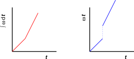
| θ = | ∫ | ω dt (27) |
which is equal to (ω t) if ω is constant, but generally not otherwise.
The physical significance of this can be appreciated with the help of figure 5, which compares ∫ ω dt to ω t. In both plots, ω=1 at early times, and ω=2 at later times. You can see that changing ω in the expression ω t produces a large unwanted “leverage” effect, with a lever-arm of length t.
The same conceptual issue arose in section 1.1. The same issue arises in many other contexts, including the frequency modulation that one encounters in radio electronics and other signal-processing applications.
This document incorporates many insights and suggestions from the members of the phys-l discussion list.