Weight, Gravitational Force, Gravity, g,
Latitude, et cetera |
* Contents
1 Weight
1.1 Definitions
The weight of any simple object is a vector W and is defined
as:
|
W := m g | |
| (in some chosen reference frame)
| |
| (1)
|
where m is the mass of the object; see reference 1 for a
discussion of how to define “mass”. Meanwhile, g is the vector
representing the local gravitational acceleration. We define g as:
|
g := the acceleration of a freely-falling test particle | |
| (relative to some chosen reference frame)
| |
| (2)
|
Equation 1 says nothing about what may be causing the
local gravitational field. The definition of g does not care
“why” the free objects are accelerating. The only thing that
matters is the phenomenological fact that they are accelerating. See
section 2.2 for a discussion of physical processes that can
produce a gravitational field, including place-to-place variations in
the gravitational field.
Both W and g are frame-relative, as can be seen by comparing
item 1, item 2, and item 3 in section 1.2.
1.2 Basic Properties
-
- 1.
In the terrestrial “laboratory” reference frame,
the largest contribution to g can be calculated from the size and
mass of Planet Earth, by means of Newton’s law of universal
gravitation (equation 9). However, that is
definitely not the only contribution to g in the lab frame, for
reasons discussed in section 3.1.
- 2.
A pencil in an orbiting spaceship is weightless
according to an observer in the ship’s reference frame. For more on
this, see section 5.
- 3.
Meanwhile, the orbiting pencil is not weightless
according to an observer in a ground-based reference frame. Let’s be
clear: it is the frame that matters. The pencil does not become
weightless because of the motion of the pencil, but because of the
motion of the reference frame.
Mass is 100% independent of the choice of frame.
Weight is 100% dependent on the choice of frame.
|
|
|
|
- 4.
Notation: Note the following contrast:
|
In this document, the weight vector is denoted by W, with
no boldface or other decorations. The scalar magnitude of W is
denoted by |W|. (It is not worth the trouble to come up with a more
compact notation for |W|.) This convention works fine for all
media, including handwritten notes, books, email, and so forth. This
convention is consistent with – and practically required by – more
advanced work involving multivectors. See reference 4
for more on this.
|
|
Many books represent vectors using boldface
symbols such as W, and use the corresponding non-boldface symbol to
represent the magnitude of the vector: W ≡ |W|. That
convention works OK for books and for web pages, where boldface is
easy to achieve, but when you’re writing things by hand it is not very
convenient. Some other books write little arrows over vectors. Both
of these conventions become inconvenient or outright impossible when
multivectors are involved.
|
For these reasons, among others, the smart policy is to write vectors
without any decoration, i.e. without boldface, without arrows over
them, without lines under them, or anything like that.
Keeping track of what’s a vector and what’s not is no different from
keeping track of the dimensions. Vectors do not require special
notation. In complex documents, it may help to include a legend or a
glossary, to systematically document what the various symbols mean.
- 5.
The W and g vectors are directed downward.
I don’t think of this as part of the definition of W
or g; instead, I think of it as the definition of “downward”.
- 6.
Since g is a vector, it is improper to ask
whether it is positive or negative. There is no “greater-than”
relationship defined for vectors (except possibly in one-dimensional
vector spaces, which we exclude from consideration, since we are
interested in multi-dimensional motion). Therefore you can’t ask
whether a vector is “>0” or “<0”. Of course for any vector
g, the magnitude |g| is non-negative, but that doesn’t tell us
anything we didn’t already know (since the magnitude of any
vector is necessarily non-negative).
Therefore, when folks ask about the sign of g, you know they
are asking an unanswerable question. It is often difficult to figure
out what prompted the question, but here are some hypotheses
for you to consider:
-
Sometimes they intended to ask about some particular
component of g in some chosen reference frame. The answer
could be positive or negative, depending on what basis vectors
they have chosen. If the +Z basis vector points downward, then gz is
positive, whereas if the +Z basis vector points upward, then gz is
negative. This is a common source of confusion, because everyone
is free to choose whatever basis they like.
- Sometimes they intended to ask about projection of g along the
direction of some other physically-significant vector in the problem.
Again this depends on which other vector they’re talking about,
but at least the answer to this question is physically-meaningful and
observer-independent, once the question has been spelled out in
sufficient detail.
- Also: when people seem to be confused about the “sign” of g,
often the main problem lies elsewhere. It may have to do with velocity
versus speed, as discussed in reference 5.
- 7.
Some people prefer to speak of the force due to
gravity (or the force “of” gravity) instead of weight. Similarly
they prefer to denote it Fg instead of W. (Usually Fg means
exactly the same thing as W.) This allows us to write
nice expressions such as:
|
Fg | | := | | gravitational force |
| ag | | := | | local gravitational acceleration |
| Fg | | = | | m ag
|
| (3)
|
without even mentioning weight, as opposed to
|
W | | := | | weight, i.e. gravitational force |
| g | | := | | local gravitational acceleration |
| W | | = | | m g
|
| (4)
|
Equation 3 has the advantage of logic and elegance, but it
hasn’t caught on very widely.
- 8.
Most people live placidly near the surface of the
earth, where |g| is constant within 1% or so, which means there is,
rougly speaking, a one-to-one correspondence between weight and mass.
This explains why non-experts commonly blur the distinction between
weight and mass.
However, the distinction remains important, and will never die out.
For example, as previously mentioned, it is very convenient to say
that astronauts are weightless (relative to the spaceship) but not
massless.
Also, for careful work, you need to take into account the fact that
|g| depends on where you are on the earth’s surface. The variation
is on the order of one percent. See reference 6.
- 9.
The weight of an object in the lab frame will be
very slightly time-dependent for various reasons including
weather-related changes in the mass of air overhead, solar gravity,
lunar gravity, et cetera.
- 10.
I find it unhelpful to define or recognize any
distinction between “true weight” and “apparent weight”.
Weight is weight. Let’s just call it the weight. If the
weight relative to one accelerated reference frame is different from
the weight relative to another, so be it. The situation
is symmetrical; there is no basis for deciding which weight is
“true” and which is “apparent”. Even if you could decide
that one frame is “true” and the other only “apparent”,
what are you going to do when there are three mutually-accelerated
frames?
- 11.
The word “gravity” is ambiguous, because it could
refer to the gravitational potential, the gravitational acceleration,
the tidal stress, et cetera. Except in cases where the details don’t
matter, or are obvious from context, it is better to avoid the word
“gravity” and use some more specific term instead.
Note that the term “gravitational field” by convention refers to the
gravitational acceleration, even though the gravitational potential is
also a field (in accordance with the usual definition of “field”).
Similarly the tidal stress is a field.
- 12.
Even if we confine attention to things with dimensions of
acceleration, there remain some very important ambiguities. Some
more-explicit, less-ambiguous terminology is discussed in section 2.
- 13.
The weight will not in general equal the total
downward force. Weight includes only the force due to the local
gravitational field, not the forces due to buoyancy, air currents,
magnetic fields, bungee cords, or anything else. However, in a fair
number of practical situations we can arrange that these
non-gravitational contributions are negligible, in which case the
weight can be well approximated by measuring the total downward force,
perhaps by letting the object rest on a spring-scale. (Assuming
of course that the scale itself is at rest in the chosen reference frame.)
It is important to use the right type of scale, because some scales
are primarily sensitive to weight (i.e. force), some scales are
primarily sensitive to mass, and some are sensitive to some weird
combination of the two. (Scale manufacturers can get away with
considerable vagueness, since they assume their scales will be
operated on the Earth’s surface, where |g| is reasonably uniform and
well-known. See section 6.3.)
- 14.
Similarly, there some grade-school textbooks
that try to define weight (not just approximate it) by saying
weight is “whatever the scale reads”. Such a definition cannot be
taken seriously, for a number of reasons. The problems
include:
- This is an “instrumental” definition. Like all instrumental
definitions, it is open to all sorts of questions about what happens
if the instrument is miscalibrated, or outright broken. There are
serious philosophical questions here, and also nontrivial practical
questions when we start asking about your weight on the moon, or your
weight aboard a space station, since scales that behaved fine on the
earth might well misbehave in other situations.
You might try to solve this class of problems by talking about an
“ideal” scale, but defining what you mean by that is no easier
than defining “weight” from scratch.
- If you were to take the scale reading literally, you would
be in error, because you would have neglected the buoyancy
correction.
- Almost all scales are intended to measure mass, not
weight. For example, consider kitchen scales. If the cookie recipe
calls for 1/4 pound of butter, the intention is presumably to
use the same mass of butter even if I am baking cookies on the moon.
- In practice it is not particularly uncommon to find two scales
in the same room, one of which (to a good approximation) responds to
mass (m) while the other, to a good approximation, responds to
weight (mg).
- Perhaps the most serious objection is that this notion of weight
applies only to objects that are stationary or at least
unaccelerated relative to the scale. For objects that are free
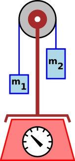
to move, indeed even partially free to move (such as an Atwood
machine, as shown in figure 1, or even a simple
pendulum), the true weight is still there, as evidenced by the
acceleration of the object, but the actual force exerted on the scale
will not be equal to the weight mg.
A student on a scale, hopping up and
down, will illustrate the same point, namely a scale-reading that is
wildly time-dependent and therefore different from what we would like
to call “the” mass or “the” weight.
Another notorious example is an hourglass on a scale. The flow of the
sand causes the center of mass of the hourglass to move downward. In
some rare cases, the motion of the center of mass will be uniform (to
a sufficient approximation) in which case it doesn’t affect the
reading. In other cases, depending on the shape of the sand-chambers
and other factors,
the motion of the center of mass will be
nonuniform. This counts as an acceleration of the hourglass as a
whole, in which case the situation is analogous to
figure 1, and the force on the scale will not be equal
to the weight mg.
Bottom line: Defining weight in terms of whatever “the” scale reads
runs a large (and quite unnecessary) risk of spreading misconceptions.
2 Various Different Notions of “Gravity”
2.1 Extrinsic, Framative Gravity
The word “framative” is a contraction for “frame-relative”. We
now restate equation 1, representing the framative
weight and the framative gravitational acceleration using more-explict
notation:
where the subscript “@f” means “relative to f”, where f is
some chosen reference frame.
In situations where it is obvious from context which reference
frame is intended, it is conventional to write simply g as shorthand
for g@f, and to call it “the” gravitational field. However, as
always, shorthand entails some risk. When in doubt, use the more
explict notation, g@f.
It must be emphasized that different frames will have different
g-values. This can happen even if both of the frames cover a single
region. The g-value depends on what the frame is doing, not on what
any particular particle is doing. To illustrate this point, consider
two objects and two frames, making four cases altogether:
falling object,
elevator frame
g@E = 0
|
|
falling object,
lab frame
g@L = 9.8 m/s/s
|
object on desk,
elevator frame
g@E = 0
|
|
object on desk,
lab frame
g@L = 9.8 m/s/s
|
where @L refers to the lab frame, and @E refers to frame comoving
with the elevator. In this example, the desk is stationary in the lab
frame, while the elevator is in free fall.
The framative gravitational field g does not have to be the same
everywhere. Suppose we have a bear located at the north pole, a
penguin located at the south pole, and a troll located in a small
hollow space at the center of the earth. Then the gravitational field
g at these locations, measured relative to the earth-centered
earth-fixed reference frame, is
|
| | g@ECNR(bear) | = | −9.8 | m/s/s x^ |
| a@ECNR(bear) | = | 0 | |
| g@ECNR(troll) | = | 0 | |
| a@ECNR(troll) | = | 0 | |
| g@ECNR(penguin) | = | 9.8 | m/s/s x^ |
| a@ECNR(penguin) | = | 0 | |
|
(6) |
where @ECNR refers to an earth-centered non-rotating reference
frame, and x^ is a unit vector pointing toward the north
celestial pole, roughly in the direction of the star Polaris. In the
ECNR frame, the total acceleration a of the bear is zero, because the
downward force of gravity is compensated by an upward force from the
ice, pushing upward against his feet. Similar words apply to the
penguin. The troll is not subject to any gravitational force or any
contact force, so he just rattles around loose.
When you choose a frame, it doesn’t have to be local. For example,
consider a freely falling elevator located at the north pole. Choose
a special frame that is comoving with this elevator. The frame can be
as small or as large as you like. We can even extend it to cover the
entire earth. The bear is weightless, relative to this special frame.
Meanwhile, the penguin is subject to an acceleration of twice the
conventional terrestrial gravitational acceleration, relative to this
special frame. In more detail:
|
| | g@ffNP(bear) | = | 0 | |
| a@ffNP(bear) | = | 9.8 | m/s/s x^ |
| g@ffNP(troll) | = | 9.8 | m/s/s x^ |
| a@ffNP(troll) | = | 9.8 | m/s/s x^ |
| g@ffNP(penguin) | = | 19.6 | m/s/s x^ |
| a@ffNP(penguin) | = | 9.8 | m/s/s x^ |
|
(7) |
Here “@ffNP” refers to “freely falling at the North Pole”. The
bear is weightless in this frame, but is not in free fall. He is
subject to an upward force from the ice. This upward force is not
opposed by any gravitational force in this particular frame, so he
accelerates upwards, towards Polaris.
The penguin is subject to a strong gravitational force towards
Polaris, which is half-canceled by the force of the ice pushing on his
feet.
More generally, each of the values in equation 7 is related to
the corresponding value in equation 6 by adding 9.8 m/s/s in
the +x^ direction.
2.2 Intrinsic, Massogenic Gravity
We can use equation 6 to calculate the difference between the
gravitational field acting on the bear and the gravitational field
acting on the troll. We can also use equation 7 to calculate
the same thing, and we get the same value. In fact, we get the same
value in any nonrotating frame.
|
δg | | = | | g@ECNR(bear) − g@ECNR(troll) |
| | | = | | g@ffNP(bear) − g@ffNP(troll) |
| | | = | | g(bear) − g(troll) |
| | | = | | −9.8 m/s/s x^ |
| (8)
|
The δg on the LHS of equation 8 is the
difference between two gravitational fields. Newton’s law of
universal gravitation gives us a more general expression for
δg, namely:
where G is the universal gravitational constant, and (in this
example) M is some mass (such as the mass of the Earth), and r^ ≡ r/|r| is a unit vector in the r-direction.
Specifically, δg(R, r) is the difference between the
gravitational field at location R+r and location R, and
δgM(R, r) is one contribution to this difference, namely the
contribution from a mass concentrated at location R. The result is
the same for any R, so the R drops out, and we write the shorthand
expression δgM(r).
We call δgM the massogenic contribution because it is
proportional to the mass M. In a non-rotating frame, contributions
of this form will be the only contributions to δg. However,
in a rotating frame, there will also be a centrifugal contribution.
(The procedures for dealing with rotating reference frames in general,
and centrifugal fields in particular, are discussed in reference 7.)
The RHS of equation 9 is manifestly
frame-independent. It should be clear from section 2.1 that
there cannot be any frame-independent expression for g(bear)
or g(troll) separately, but we can have a frame-independent
expression for the difference between the two. The difference is
proportional to the mass of the planet, and inversely proportional to
the square of the distance.
Strictly speaking, equation 9 applies only to a
small, localized mass. It applies in the “classical” limit, which
requires that the fields must be not too strong and not too rapidly
changing. It also requires that the mass M must be not too rapidly
spinning. These requirements are satisfied in the solar system, with
a wide margin of safety for all practical purposes. In a
non-classical situation, equation 9 must be replaced
by the equations of general relativity.
There is a theorem due to Newton that says that if you are outside a
uniform spherical shell of mass, its contribution to the gravitational
field is the same as if all the mass were concentrated at the center.
If you are inside such a shell, its contribution to the gravitational
field is zero. Therefore, to the extent that a planet can be
considered to be made up of a series of concentric shells, where each
shell has a uniform density, then equation 9 applies
directly and simply. The mass on the RHS is the total mass.
On the other hand, if the planet is not isotropic, equation 9 can still be applied, but brute force is
required. The procedure is to break the planet into a great number of
small regions, apply the equation to each region separately, and then
add up all the contributions to the field.
2.3 Digression: Standard Gravity
There is one more notion of “the” gravitational acceleration that we
should mention. As will be discussed in section 6.1, the
“standard” acceleration of gravity is defined by fiat to be 9.80665
m/s2 exactly, and is denoted gN. The direction is unspecified.
This gN is useful as a benchmark, as a standard of comparison. The
actual value of |g@L| at sea level in temperate latitudes is close
to gN, with a small fraction of a percent.
2.4 Discussion
- The local framative gravitational acceleration g@L is what
matters to an apartment building or a grandfather clock or anything
else that sits in one place near the earth’s surface. Therefore g@L is “the” gravitational acceleration relevant to architects and
clockmakers.
- In contrast, the massogenic contribution δgM(r) is
“the” gravitational acceleration relevant to astrophysicists. You
can get away with setting g = δgM if there is only one
large mass in the problem, and you always choose an unaccelerated
non-rotating reference frame centered on the mass M.
- In many situations, there is a choice, and different people
could reasonably choose differently. For example, when analyzing an
orbital rendezvous maneuver, you could choose an earth-centered
non-rotating frame, or an earth-centered earth-fixed co-rotating
frame, or a frame comoving with one of the spacecraft. The g-value
will be different in each case. The only sane path forward is to be
explicit about what frame is being used.
- Beware: Many introductory-level physics textbooks use
inconsistent terminology, switching back and forth from one
definition to another. In the chapter on universal gravitation,
“g” and “gravitational acceleration” probably refer to the
intrinsic, universal, incremental field, δg. Meanwhile, in
other chapters, including anything related to practical weighing,
“g” and “gravitational acceleration” almost certainly refer to
the extrinsic framative field, g@L.
- Note the sun’s gravitational field differs in direction and
magnitude as you go from place to place on earth. This difference in
gravitational field gives rise to something we call tidal
stress, which indirectly drives the observed tides.
The same idea applies to the intrinsic, universal, incremental
δg. It is a difference in gravitational field between
one place and another, so in some fundamental conceptual sense, it is
tidal.
- As you may have heard, general relativity explains
“gravitation” in terms of the curvature of spacetime. It must be
emphasized that curvature has to do with the intrinsic δg.
The curvature of spacetime produces tidal stress. Curvature has got
absolutely nothing to do with the local, extrinsic, framative g.
See reference 8 for a simple description of how this works.
3 Some Common Reference Frames
We now consider various reference frames that are commonly used, and
discuss some of the physical processes that contribute to the value of
the framative g in each frame.
3.1 The Terrestrial Laboratory Frame
The gravitational acceleration in the ordinary lab frame is denoted
g@L, where the L stands for laboratory.
As always, g can be measured by dropping an object and measuring its
freely-falling motion relative to the laboratory ... or by weighing a
known mass. Considerable accuracy can be achieved, relatively easily,
using a reversible pendulum (Kater pendulum, or something along those
lines). See reference 9.
In the lab frame, g@L includes the following contributions:
-
The universal gravitation term, δg(r, M), where M is the mass
of the earth. This is far and away the largest contribution to
g@L.
- The centrifugal field of the earth’s rotation.
- The fact that the earth is generally oblate rather than
spherical, as a consequence of the aformentioned centrifugal field.
This changes the radius-vector r that appears in the law of
universal gravitation and in the centrifugal-force law.
- Topographic elevation, which also changes r.
- Local variations in the density of the earth.
- The direct and indirect effects of lunar gravity, including the
monthly motion of the earth around the center-of-mass of the
earth/moon system.
- The direct and indirect effects of solar gravity, including the
annual motion of the earth around the center-of-mass of the
earth/sun system.
- Weather-related variations in the mass of air overhead.
- Various smaller terms.
To repeat: The difference |g@L − δg(r, M)| is not zero. It is usually
less than 1% of |g@L| but not much less, depending on latitude,
elevation, et cetera.
3.2 Earth-Centered Nonrotating Frame
We can with a little effort construct a situation where the actual
gravitational acceleration g is very nearly equal to δg(r,
M). One possibility is suggested by figure 2.
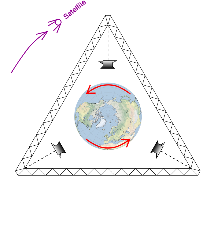 Figure 2
: Earth-Centered Nonrotating
Reference Frame
As shown in the figure, we imagine a huge triangular truss has been
constructed in space high above the equator. The center of the truss
coincides with the center of the earth. It must be emphasized that
the truss is not orbiting i.e. not rotating. Such a frame is called
an earth-centered nonrotating (ECNR) reference frame.
Observers on the truss observe that the earth spins below them once
every sideral day.
The ECNR frame is sometimes convenient for analyzing the motion of a
satellite in earth orbit.
In this reference frame, the weight of the anvils (as shown in the
diagram) is very nearly given by equation 9. That
is, m g is very nearly m δg(r, M). All of the correction
terms mentioned in section 3.1 must still be considered,
which means that the ECNR frame is not exactly an inertial frame.
- We have gotten rid of the centrifugal term because
the frame is not rotating.
- We don’t need to worry too much about the oblateness
because we are measuring things relative to the center of
the earth, not relative to the surface
- The satellite is sufficiently high that it is not very sensitive
to the details of the earth’s geology and geography.
- The ECNR frame is “almost” inertial. That is, the correction
terms are fairly small. For example, the acceleration of the earth
in its annual orbit is only 0.06% as large as the earth’s surface
gravity. That’s 600 parts per million.
The remaining correction terms are on the order of a few parts per
million, or smaller.
3.3 Proper Weight
For a rigid object, its proper weight is the mass times the proper
acceleration gp. This refers to g as measured in a frame
instantaneously comoving with the center of mass of the object. This
is an elegant and sophisticated idea, and is sometimes very useful.
For example, proper acceleration is essential if you are designing an
inertial guidance system. For details, see
reference 10.
On the other hand, proper weight is not appropriate for an
introductory discussion of gravity and weight. For one thing, it
blurs the distinction between the motion of the frame and the motion
of the object. Secondly, if the frame is undergoing nonuniform
acceleration, this introduces complexities into the laws of motion,
which introductory-level students are not prepared to handle.
Thirdly, there are subtleties in the definition of proper
acceleration. Obviously you can’t think of an object as accelerating
relative to itself, but nevertheless proper acceleration is a
well-defined concept.
3.4 Car, Aircraft, Spacecraft, etc.
For an observer traveling in a vehicle – perhaps a car, aircraft, or
spacecraft – it is very common to use a frame of reference that is
instantaneously comoving with the vehicle. There are many advantages
to doing so. There is however some cost to doing so, because if the
vehicle’s reference frame is accelerating or turning, this must be
included in the definition of the vehicle’s framative gravitational
acceleration, g@V.
For a car moving in a straight line relative to the laboratory, g@V and g@L will be the same. In contrast, if the car is zooming
over the crest of hill, or if it is making a sharp turn, g@V and
g@L will be significantly different.
3.5 Other Frames
The examples mentioned so far are definitely not the only g-like
quantities that can be defined. For starters, you can define 2N
different g-like quantities just by selectively including or
excluding the “corrections” mentioned in section 3.1.
4 The Direction of g; Vertical and Horizontal
As mentioned in section 3.1, the lab-frame weight m g@L is
approximately but not exactly equal to m δg(r, M). In theory, m
g@L would exactly equal m δg(r, M) for the lab frame on an isolated
airless nonrotating spherical homogeneous planet, but there aren’t any
of those around here.
In this section we consider the direction of the gravitational
acceleration vector; if you are interested in the magnitude, see
section 5.
The direction of our lab-frame gravitational acceleration vector is
consistent with the conventional notions of vertical and horizontal.
A table in the laboratory is considered horizontal if things don’t
spontaneously roll off it, which is dependent on g@L (not gN
or δg(r, M)).
The surface of a liquid at rest is an isopotential surface, locally
and globally. The local orientation of this surface defines what we
mean by horizontal. That is to say, the ordinary notion of “sea
level” does not makes sense unless we include centrifugal terms in
our notion of gravity. Operationally, this means that an undisturbed
pool of water is horizontal, and an undisturbed plumb line is
vertical.
The angle between the vectors g@L and δg(r, M) is about 0.1 degrees at
temperate latitudes.
Here’s a parable: Once upon a time, some folks who misunderstood the
distinction between g@L and δg(r, M) decided to build a swimming pool.
It was 50 feet across. They wanted the rim of the pool to be
horizontal, but they constructed it to be perpendicular to δg(r, M)
rather than to g@L, based on careful astronomical observations. As
a result, one side was just over one inch too high, measured relative
to the water. This looked really terrible. The point of the story is
that in accordance with the laws of physics, the water distributed
itself according to g=gE=g@L, not δg(r, M).
To summarize: in practical terrestrial applications, the gravitational
acceleration is not equal to GM/r2. In addition to the
GM/r2 term it includes the centrifugal term and various smaller
corrections. This result does not depend on any sophisticated notions
of modern physics. In particular, we do not need to invoke Einstein’s
principle of equivalence (although we could). Instead we are
depending on basic, practical, operational notions of horizontal,
vertical, up/down, and gravity – notions that predate Einstein and
predate Newton by thousands of years.
On the other side of the same coin, our approach is entirely
consistent with modern physics notions. We say that g means gE,
and and includes all contributions to the acceleration of the
reference frame, relative to free fall. This is as it should be in
accordance with Einstein’s principle of equivalence, which asserts
that a gravitational field is locally indistinguishable from
acceleration of the reference frame.
5 The Magnitude of g; Weightlessness
This brings us back to a point made earlier: even though mass is 100%
independent of the choice of reference frame, weight is 100%
dependent on the choice of reference frame.
In this section we consider the direction of the gravitational
acceleration vector; if you are interested in the direction, see
section 4.
The magnitude of g@L differs from the magnitude of δg(r, M) by about
one third of a percent at the equator, and about one quarter of a
percent at temperate latitudes. This would be very significant
in ordinary laboratory practice if you used a scale that
measured weight ... which is why laboratory scales are
generally designed to measure mass, not weight. For
example, a two-pan balance compares one mass with another
in a way that is insensitive to small changes in |g|.
The sensitivity of the balance depends on |g|, but
the balance-point does not.
It turns out that variations in the direction of g
are often more interesting than the variations in the
magnitude.
Important examples
include:
-
In the usual terrestrial lab frame, the dominant contribution to
g@L is δg(r, M), with significant corrections due (directly and
indirectly) to the centrifugal field associated with the earth’s
rotation.
- Astronauts living in a space station correctly consider
themselves weightless, because they are using a frame comoving with
the spacecraft, and restricting attention to regions near the
spacecraft. In that frame (and in those regions), g is millions of
times smaller than gN.
6 Units and Measurements
6.1 Definitions of Units
The conventional “standard” gravitational acceleration is by
international agreement defined to be 9.80665 m/s2, and is called
one Gee, often shortened to just G. According to NIST, the
recommended symbol is gN but everybody I know calls it Gee or G
(not to be confused with Newton’s constant of universal gravitation,
also denoted G).
This gN is useful for calibrating accelerometers in a standard way.
It was never intended to tell you the actual g@L of your
laboratory.
The actual observed gravitational acceleration in an earthbound
laboratory is typically within 1% of the “standard” value, but of
course varies with time, location, elevation, et cetera. Reference 6 provides a tool for looking up measurements of the local
gravitational acceleration almost anywhere in the United States.
The kilogram (kg) is defined to be a unit of mass. There also
exists an informal unit, the “kilogram of force” (kgf), which
is defined to be one kg multiplied by one Gee.
The pound (lb) is a unit of mass. The pound has been in use
since the late 13th century or early 14th century. That means the
idea of “pound” is hundreds of years older than the idea of
“F=ma”. (In contrast, the “kilogram” is more than a century
younger than “F=ma”.)
Some people claim the pound (as used in the US) to be defined as a
unit of force, but this is not true. As far as I can tell, it has
never been true. Under US law, the pound has been recognized as
proportional to the SI unit of mass – the kilogram – since 1866.
Under US law from 1901 to 1959, the pound was explicitly defined in
terms of the kilogram, namely 0.4535924277 kg. By international
agreement adopted in 1959, the “international pound” is defined to
be 0.45359237 kg, which is now the value used for all purposes in the
US. See reference 11 and reference 12.
There also exists, informally, the “pound of force” (lbf), which
is defined to be one lb multiplied by one Gee. If you hear somebody
talking about a “pound of weight”, you can assume they mean lbf.
In general, though, lbf should be avoided. Some constructive
alternatives are discussed in section 6.2.
Scientists who measure the variations in the earth’s gravitational
field customarily use units of gals and milligals. The gal is defined
to be 1 cm/s2, so it is 100 times smaller than the SI unit of
acceleration. The gal is named in honor of Galileo, but gal is the
full name of the unit, not an abbreviation. Conversely, there
is no abbreviation for gal. The abbreviation for milligal is mgal.
If you are doing unit-conversion calculations using
the “units” program, the gal unit must be capitalized, i.e. Gal.
This non-standard capitalization is a kludge to avoid conflict with
the even-more-non-standard abbreviation for gallon.
6.2 The Effect of Units on the Form of Laws
SI (Le Système International d’Unités) was designed so that most
of the units are consistent with each other, and consistent with the
laws of physics. For example, the SI unit of force is equal to the
unit of mass times the unit of acceleration, so we can write F=ma
without any conversion factors.
Other systems of units are not always so consistent, in which case you
must re-think many of the laws of physics, with an eye toward putting
in conversion factors where needed. For example,
-
If you want to measure acceleration in feet per second per
second, mass in lb, and force in lbf, then you cannot write
the second law in the form F = m a. Instead you must write
F = m a/g. This is what I usually do, on the rare occasions when
I am forced to calculate with pounds at all.
- If you want to measure mass in lb and force in lbf, and still
write F = m a without a conversion factor, then you must measure
acceleration in Gees (not in feet per second squared). This is almost
equivalent to the previous option; it just absorbs the conversion
factor into the definition of acceleration.
- If you want to measure acceleration in feet per second per
second and mass in lb, and still write F = m a, then you must
measure force in poundals.
- Some older engineering books measure force in lbf,
mass in slugs, and acceleration in feet per second per second.
This allows them to write F = m a without a conversion factor.
- My advice is to convert everything to SI at the first
opportunity, so we can forget about ugly things like poundals and
slugs.
6.3 Instruments
Note the contrast:
|
Some instruments measure mass. These are
typically labeled in kg and g, or lb and oz ... which makes sense.
|
|
There are other instruments that measure force. Unfortunately, these
are often labeled in mass units (such as kg) when they should be
labeled in force units (such as kgf).
|
As if things weren’t complicated enough, sometimes you find
instruments that measure some weird linear combination of mass and
weight. They might use a balance (mass) to obtain the high-order
digits of the reading, and then use a spring (force) to obtain the
low-order digits. Fortunately though, under standard conditions on
the earth’s surface, it usually doesn’t matter very much whether the
instrument measures true mass, true force, or some combination
... since mass and force have a known proportional relationship under
standard conditions.
However, it is interesting to ask whether such-and-such instrument would
work correctly on the surface of the moon, or in the weightless
environment of a space station. Actually that’s not quite the right
question, since whether the instrument “works” depends partly on the
instrument but also depends on how you choose to use the instrument.
For any instrument, you can pull on it with a rubber band (or magnet
or whatever) in such a way that you are almost certainly measuring the
force of the rubber band, not the mass of the rubber band. On the
other hand, for any instrument, you can hook up a passive object in
such a way that you are measuring the mass of the object.
In non-standard conditions, such as on the surface of the moon, a
balance-type instrument is good for measuring mass. It can measure
mass without needing to be recalibrated. However, it is a disaster for
measuring force. Conversely, a spring-type instrument is good for
measuring force, but is a disaster for measuring mass.
As Michael Edmiston has pointed out, there is a large class of
mass-measuring instruments (including some of the crudest, and also
many of the finest) that contain a built-in standard of mass, and
measure things relative to this standard. Instruments in this class
can be expected to measure mass (not force, not weight), independent
of the value of |g| over some reasonably-wide range.
The interesting thing about such instruments is they assume that g
is not changing too much as a function of time, and/or assume g is
not changing too much as a function of position. That is:
-
A beam-balance compares the mass in one pan against a standard
in the other pan. This can measure mass extremely accurately, but is
subject to the assumption two pans are located sufficiently close
together that there is no significant difference in g between the
two locations.
- Likewise, some very fine laboratory-grade single-pan instruments
use a force sensor, but calibrate it against a standard mass every so
often. This also can measure mass extremely accurately, but is
subject to the assumption that g doesn’t significantly change
between the time of the calibration and the time of the
measurement.
7 Latitude
Because of the earth’s centrifugal field, and for other reasons
discussed in section 3.1 and especially section 4, the conventional “down” direction does
not point toward the center of the earth. So you might be
wondering how to measure the difference between these two directions.
First let me outline a seemingly plausible measurement scheme
and explain why it does not answer the question:
-
Use a sextant to measure the height of the celestial pole
above the horizon, and compare that to your latitude.
- Equivalently, perhaps more accurately, use a sextant to
measure what stars are overhead, and compare their declination
to your colatitude.
As it turns out, that scheme doesn’t work, because by tradition the
“latitude” is defined to be the geodetic latitude, i.e.
defined to match what you see in the sextant! It is defined in terms
of the local notion of horizontal and vertical, which includes the
centrifugal acceleration. All that makes sense if you think about how
latitude has been used for navigation over the centuries.
To say the same thing the other way, the unadorned term “latitude”
does not correspond to the geocentric latitude, i.e. the angle
as seen from the center of the earth.
As a consequence of the definition, parallels of latitude are not
equally spaced. This is easy to visualize if you extrapolate to a
planet with extreme flattening, so that the geoid looks like a
pancake.
So, if you want to measure what’s going on, it requires nothing more
than a highly accurate map, or (preferably) accurate survey data.
Measure the north-south distance between two points, and compare it to
the difference in latitude. Do this twice: Once for a pair of points
near the equator, and again for pair of points far from the equator.
You can simulate the experiment using a good geodesy software package.
Beware that there are some not-so-good packages out there. I haven’t
done exhaustive checks, but so far I’ve been happy with
GeographicLib by
Charles Karney.
I calculate that one degree of latitude is
|
111.694 km | | | | near the pole |
| 110.574 km | | | | near the equator
|
| (10)
|
8 That Falling Sensation
Reference 13 addresses the bodily feelings
associated with free fall, weight, and/or weightlessness.
9 The Figure of the Earth
The earth is not a sphere. To a good approximation, it is an
ellipsoid. That is the natural shape for a spinning, gravitating
object in mechanical equilbrium. A wonderful review can be found in
reference 14. It outlines the contributions of Newton,
Maclaurin, Jacobi, Meyer, Liouville, Dirichlet, Dedekind, Riemann,
Poincaré, and Cartan.
It is well known that the gravitational field is less at the equator
than at the poles. The variation is not huge, but it is nontrivial.
It is easily measurable using simple instruments, especially if you
measure it at widely-separated places and compare notes. If you wish
to calculate this from first principles, you should follow the recipe
given in reference 14. The general case requires evaluating
lots of spherical harmonics, but when the ellipsoid is not very
eccentric, things are a lot simpler.
In contrast, it would not correct to treat the
earth as a point mass and calculate the field using only the
universal massogenic formula, equation 9. It’s
tempting to try that, because the radius is greater at the equator,
so you might think the weaker field is explained by the 1/r2
dependence in equation 9 ... but that’s not the
correct physics. It’s not even close. It overestimates the
effect. That’s because there’s more stuff under your feet at the
equator, and less at the poles.Newton showed that the field of a uniform spherical object is
the same as you would get from a point mass at the center ... but
he also showed that the same cannot be said of an ellipsoid.
Also it would not be correct to neglect the centrifugal field.
The usual terrestrial lab frame is a rotating frame, and the
observed g in that frame contains a smallish but nontrivial
contribution from the centrifugal field.
Figure 3 shows some data, and compares it to various
models. The black circles are calculated using the EGM2008 model,
evaluated at various locations around the globe. The model is based
on thousands of measurements, and uses thousands of adjustable
parameters, so it should be pretty good. I checked the model against
one actual direct measurement (Blackford Hill) and it agreed quite
closely. The scatter in the data is presumably due to inhomogeneities
in the earth, as a function of longitude. The red circles are from
reference 15; I have no idea whether they are based on a model
or direct measurements.
All the plotted points are corrected to sea level. If you want the
actual measured acceleration at any location, starting from figure 3, you need to apply an elevation correction.
The EGM2008 model can be evaluated as a function of latitude,
longitude, and elevation using the Gravity program which is part of
the Geographiclib suite.
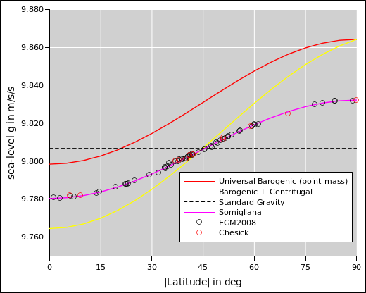 Figure 3
: Gravity as a Function of Latitude
The dashed black line shows the plain old “standard” gravity. It’s
a good approximation if you live in Ottawa, Seattle, or Paris ... but
not so good if you live at a significantly higher or lower latitude.
The red curve is what you would get by treating the earth as a point
mass and calculating the field on the surface of the ellipsoid,
plugging the geocentric radius into equation 9.
The yellow curve is what you would get by combining the universal
massogenic contribution plus the centrifugal contribution. It is in
the right ballpark in the mid-latitudes, as you might expect ... but
at higher or lower latitudes if you want a decent result, you have to
move beyond the point-mass approximation. That is, you need to
account for the fact that there is more stuff under your feet at the
equator than at the poles.
Last but not least, the magenta curve is equation 11, the
Somigliana equation. This could be considered an empirical
three-parameter fit, fitting the gravity data as a function of
latitude, without regard to longitude. It fits the data remarkably
well for such a simple model. However, it’s even better than that,
because it is not entirely an empirical model. It’s well founded in
the physics, or at least it would be for a star or planet where the
surface was a gravitational equipotential, as the earth would be
without the dry land – and especially without the mountain ranges.
The equation is:
where φ is the geodetic latitude, g(0) is the gravitational
acceleration at the equator, e is the eccentricity, and k is a
parameter that has to do with the density distribution. The earth has
a k value greater than 0, which indicates it is denser on the inside
than it is near the surface.
For a fluid with uniform density, the problem would be
overconstrained, since we get to measure both the radius and the
gravitational field as functions of latitude. We can get a lot of
mileage out of the fact that the fluid surface has to be an
equipotential. For the real earth, the radius and field measurements
suffice to firmly reject the uniform-density hypothesis.
There are other three-parameter fits on the market, such as the
International Gravity Model, but they aren’t any simpler don’t work as
well as the Somigliana equation, and are less well founded in the
physics.
See reference 16 for the spreadsheet used to
produce figure 3. It contains the data and some
other gravity-related calculations.
If you want some data but don’t feel like installing the Geographiclib
package, there are web apps such as reference 17 or
reference 18 that will give you the g value at arbitrary
locations. Also, you can find g values for selected locations on
the appropriate page in reference 16, or in a
simpler format in reference 19.
10 Gravitational Waves
This is a very complicated subject. Reference 20 discusses some of the key concepts and
attempts to dispel some of the most pernicious misconceptions.
11 References
-
-
John Denker,
“How to Define Mass”
www.av8n.com/physics/mass.htm -
T.M. Niebauer, G.S. Sasagawa, J.E. Faller,
R. Hilt, and F. Klopping
“A new generation of absolute gravimeters”
http://www.microglacoste.com/pdf/newgeneration.pdf -
John Denker
“Simple Accelerometer”
www.av8n.com/physics/accelerometer.htm -
John Denker,
“Introduction to Vectors”
www.av8n.com/physics/vector-intro.htm -
John Denker,
“Velocity, Speed, Acceleration, and Deceleration”
www.av8n.com/physics/acceleration.htm -
GEON project,
“GeoNet Gravity and Magnetic Dataset Repository”
http://www.geongrid.org/index.php/gateways/gravitymagnetics -
John Denker,
“Motion in a Rotating Frame”
www.av8n.com/physics/rotating-frame.htm -
John Denker,
“Tabletop Geodesics, General Relativity, and Embedding Diagrams”
www.av8n.com/physics/geodesics.htm -
Wikipedia article: Kater’s pendulum
https://en.wikipedia.org/wiki/Kater’s_pendulum -
John Denker,
“Acceleration in Spacetime”
www.av8n.com/physics/spacetime-acceleration.htm -
“NIST Guide to SI Units”
http://physics.nist.gov/Pubs/SP811/appenB8.html -
Sizes Inc.,
“Pound Avoirdupois”
https://www.sizes.com/units/pound_avoirdupois.htm -
John Denker,
“Can You Feel Gravity?”
www.av8n.com/physics/gravity-perception.htm -
S. Chandrasekhar,
“Ellipsoidal Figures of Equilibrium - An Historical Account”
Communications on Pure and Applied Mathematics, xx, 251–265
(1967)
http://people.ucsc.edu/~igarrick/EART290/chandrasekhar_1967.pdf -
Elizabeth Chesick
“Acceleration due to Gravity”
http://www.haverford.edu/educ/knight-booklet/accelarator.htm -
John Denker,
“Spreadsheet for Calculating Gravity as a Function of Latitude etc.”
./gravity-centrifugity.xls
-
Andreas Lindau,
Physikalisch-Technische Bundesanstalt
“Gravity Information System”
https://www.ptb.de/cartoweb3/SISproject.php -
NIST
“Surface Gravity Prediction”
https://geodesy.noaa.gov/cgi-bin/grav_pdx.prl -
“Gravity Data from EGM2008”
./lat-lon-g.csv
-
John Denker,
“Pre-Introduction to Gravitational Waves”
www.av8n.com/physics/gravitational-wave-intro.htm