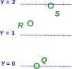
Figure 1: Some Points
Figure 1 shows some points, namely Q, R, and S.
There may be some physically-significant properties associated with each point. For example, at point R, we might be interested in the temperature T(R), pressure P(R), or something like that. We might also be interested in a point’s coordinates (relative to some given frame of reference); these could be Cartesian coordinates, polar coordinates, Minkowski coordinates, or whatever.
| We take the points to be primary and fundamental. For more about this, see reference 1. | Coordinates are not so fundamental. If we use coordinates at all, the coordinates are properties of the points. |
| The points exist as physical objects. | The points are not defined by the coordinates. |
| A given point may have one set of coordinates relative to Joe’s reference frame, and a different set of coordinates relative to Moe’s reference frame. We emphasize that this is physically the same point, no matter what the coordinates are. | A given set of coordinates in Moe’s reference frame may represent one point, while the same set of coordinates in Joe’s frame represents a different point. We emphasize that these are physically different points, no matter what the coordinates are. |
Suppose we have some property that varies from point to point in space. Usually the most effective way of understanding what’s going on is in terms of contours, such that the value of the property is constant along the contour.
As a concrete example, consider the “y” property, where y is the Cartesian y-coordinate in some reference frame. Figure 2 shows some contours of constant y, and shows where our points are situated relative to these contours.
We can easily see that y(Q)=0 to high accuracy. We can estimate the y-values of the other points, interpolating between contours if necessary.
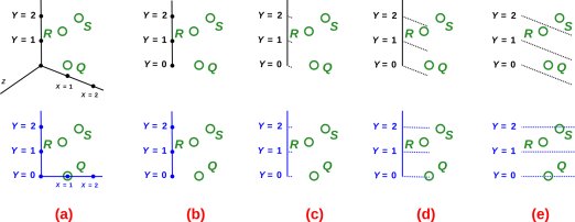
You may be wondering, where’s the y-axis? Why isn’t there a y-axis? To answer that, let’s see what’s going on in figure 3.
Proceeding left-to-right in the top row of figure 3, in column (a) we have the y-axis in context as part of an xyz triad, seen in perspective. In column (b) we have the same axis all by itself. In column (c) we use tick marks (rather than dots) to represent known y-values. In column (d) we use extra-long tick marks. In column (e) we make the tick marks even longer, so that they become purely and simply contours of constant y, and we get rid of the axis itself.
In the bottom row of figure 3, we see a similar-looking y-axis in a different context.
The idea here is that having a y-axis, even including labeled y-values on the y-axis, as in column (b) of the figure, doesn’t tell you what you need to know. If I give you such an axis out of context, you have no way of knowing whether it comes from the top row or the bottom row of the figure. And that is important to know, because in the bottom row y(S) is slightly less than 2, while in the top row y(S) is considerably bigger than 2, as you can verify by comparing the S point to the 2 contour in column (e) of the figure.
If you are given a y-axis, and want to find the y-coordinate of a point, you are in trouble unless the point happens to lie right on the y-axis, or unless you know the contours of constant y.
There is some compelling logic here: If you have the axis, you need the contours anyway ... and if you have the contours, you don’t need the axis. You can just read off the y-value by reference to the contours.
Note the contrast: The contours indicate the direction of constant y. Meanwhile, the conventional y-axis indicates the direction of increasing y. This is tricky, because there are some situations (notably thermodynamics) where there are many different directions with equally-good claims to represent increasing y. In some sense, the y axis is a contour of constant everything-except-y, but that’s not a reliable definition, because the notion of “everything-except” is not well defined.
Labeling a plot by drawing axes is more conventional, and perhaps more pleasing to the eye ... but the contours are more logical and more informative.
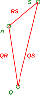
We will be interested not just in the points but also in the displacement vectors that go from one point to another, as shown in red in figure 4.
We prefer the notation χ(QS) to denote the vector from point Q to point S, but sometimes we abbreviate it as QS, as in figure 4.
These vectors have important algebraic properties. In particular, we have vector addition (i.e. adding one vector to another), vector subtraction, and multiplication of vectors by scalars. An example of vector addition is:
| χ(QS) = χ(QR) + χ(RS) (1) |
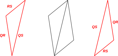
This addition is shown on the LHS of figure 5. The geometric significance of vector addition is that the addends are arranged “tip to tail” as shown in the figure.
Vector addition is commutative, so χ(QS) = χ(QR) + χ(RS) implies χ(QS) = χ(RS) + χ(QR) and vice versa. The physical significance of the latter equation is shown on the RHS of figure 5.
The geometrical rule for adding vectors is also sometimes called the “parallelogram rule” because the sum can be seen as the diagonal of a parallelogram. If you take the two red triangles in figure 5 and shove them together, you get the parallelogram shown in black in the figure. However, the parallelogram rule is simultaneously too complicated and not complicated enough. For starters, you don’t need to construct all four sides of the parallelogram; a triangle suffices to represent vector addition. Secondly, the parallelogram rule doesn’t tell you everything you need to know. To represent vector addition, you need to remember the “tip to tail” requirement anyway. The problem is that if you blindly build a parallelogram, you might build it “tip to tip” which would represent subtraction rather than addition.
It must be emphasized that displacement vectors (like the points themselves) exist as physical entities, quite independent of any coordinate system, independent of any reference frame, and independent of which observer(s), if any, are observing them. See reference 1. Think back to the “straightedge and compass” constructions that you did in high-school geometry. You can prove all sorts of geometric facts about points and vectors just using geometry, without reference to any origin, coordinate system, basis, observer, or anything like that.
Exercise: Prove the Pythagorean theorem by “straightedge and compass” methods. This emphasizes that geometry by itself is powerful; you don’t need a coordinate system to do geometry.
Also note that when we talk about the direction and magnitude of a displacement vector, we mean the direction from tip to tail, and the distance from tip to tail. In contrast, the absolute position of the vector (relative to anything else) is immaterial. That means we are free to move displacement vectors around without changing their meaning. Examples of this can be seen in figure 5, where a given vector (such as the QR vector) is depicted several times in different places … and is considered the same displacement vector in each instance.
In the previous section we discussed the geometrical and algebraic properties of the displacement vectors that run from point to point.
In contrast, we did not say much about the points themselves. For example, we did not provide any way of adding two points.
It is usually not necessary to establish an algebra for the points, but we can establish one if we want. The first step is to pick some point to use as the origin point. WLoG call it O. Then we can define the position vector of any point R to be the displacement from the origin to R. We represent this with the Roman letter x (similar to Greek χ, but not quite the same):
| x(R) := χ(OR) (2) |
Some remarks:
| (3) |
which we get by applying equation 1 to the definition equation 2. The derivative of position is similarly independent of the choice of origin, since the definition of derivative involves a subtraction.
When drawing displacement vectors, the direction of the arrows conforms to the following convention:
| R is mentioned first in χ(RS) | S is mentioned second in χ(RS) | ||
| vector “from” R | vector “to” S | ||
| tail of vector at R | tip of vector at S | ||
| negative x(R) in equation 3 | positive x(S) in equation 3 |
This means we adhere to the convention of representing displacement vectors by uphill arrows, if you think of the position as a potential. That is, the arrow points toward the positive contribution in equation 3. As a rule, displacement vectors and exterior derivatives (including gradient vectors) are conventionally drawn pointing uphill.
By way of contrast, note that electric fields are conventionally represented by downhill arrows, i.e. by the negative of the gradient of the electric potential. This carries over from physics to electronics, where the “forward” voltage drop across a resistor is conventionally shown as a vector from plus to minus, i.e. downhill down the electrostatic potential.The downhill convention often applies to other force-like fields, too.
An uphill arrow is a reasonable thing, and a downhill arrow is also a reasonable thing, but they are not the same thing. If you see arrows in a diagram, it is not a priori obvious whether they are uphill arrows or downhill arrows. For example, if we are told that figure 6 has something to do with topography, i.e. with the variation of altitude as a function of latitude and longitude, it is not particularly obvious whether the figure represents a peak or a pit.
The arrows might be gradient vectors, pointing uphill out of a pit … or the arrows might be gravitational force-field vectors, pointing downhill away from a peak, anti-aligned with the gravitational potential gradient.
In this section we temporarily assume we have a well-defined notion of “perpendicular” or “orthogonal”. This can be considered a purely geometric notion; recall that using only straightedge and compass you can construct a new line perpendicular to a given line. We also assume we can measure the length of a vector. Note that if we know how to take the dot product between two vectors, that is sufficient to define length and angle for us.
Note that it is totally nontrivial to assume that we have notions of length and angle. There are plenty of physical situations where such notions are problematic or nonexistent. For example, in thermodynamics, given a set of variable such as energy, entropy, temperature pressure, volume, etc., there is not usually any physical basis for deciding which (if any) are perpendicular to which others.
Given a notion of length and angle, we can construct a set of orthonormal vectors, as follows: Start with a list of all displacement vectors that are physically relevant to the problem at hand. Then apply the Gram-Schmidt algorithm. This removes from the list any vectors that would have been linearly dependent on earlier vectors, then makes each remaining vector orthogonal to previous vectors, and then normalizes them.
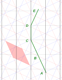
In previous sections, it was safe to assume that the points Q, R, and S lay in the Euclidean xy plane. In contrast, from now on we will be mostly concerned with spacetime, i.e. Minkowski space. Figure 7 is a spacetime diagram. The points A, B, C, D, and E lie in the xt plane (not the xy plane). The time variable t increases upwards in the diagram.
In particular, we assume that these five points happen to lie on some particle’s world-line, also shown in green in the figure.
As discussed in section 1.1 and reference 1, points and world lines exist as physical objects, independent of any coordinate system, and independent of what observers, if any, are looking at them.
Let’s deal with one small issue of terminology:
| One school of thought refers to A, B, C et cetera as events, thereby emphasizing that they each specify a time as well as a spacelike position. This emphasizes that 4 dimensions is a departure from 3 dimensions. | The other school of thought simply calls A, B, C et cetera points in spacetime. This emphasizes that 4 dimensions is not really a very big departure from 3 dimensions. |
Mostly we will speak of points rather than events. This view is simultaneously simpler and more sophisticated; we want to feel “at home” in spacetime. However, we accept the term “event” as a colorful synonym for “point” in spacetime.
In figure 7, the black lines represent the coordinates in the lab frame (aka Joe’s frame). The time direction runs upward vertically, so that the horizontal black lines are contours of constant time. The spatial x1 direction runs horizontally, so that the vertical black lines are contours of constant x1.
The red lines in figure 7 are another coordinate system, namely Moe’s coordinate system. Moe is moving to the left relative to Joe. The light-red shaded region is a timelike unit square in Moe’s reference frame. (In the diagram it doesn’t look like a square, but that’s only because the spacetime diagram-on-paper does not faithfully represent the actual geometry of spacetime. See reference 2 for more on this.)
In our example, the origin of Moe’s coordinate system coincides with the origin of Joe’s coordinate system. In particular,
| x(C) = | ⎡ ⎢ ⎢ ⎢ ⎣ |
| ⎤ ⎥ ⎥ ⎥ ⎦ |
| = | ⎡ ⎢ ⎢ ⎢ ⎣ |
| ⎤ ⎥ ⎥ ⎥ ⎦ |
| (4) |
Our example (figure 7) is constructed in such a way that points x(A) and x(B) have particularly simple representations in Moe’s frame, namely:
| x(A) = | ⎡ ⎢ ⎢ ⎢ ⎣ |
| ⎤ ⎥ ⎥ ⎥ ⎦ |
| (5) |
| x(B) = | ⎡ ⎢ ⎢ ⎢ ⎣ |
| ⎤ ⎥ ⎥ ⎥ ⎦ |
| (6) |
Simply by counting contours in figure 7, You can verify that points A and B each lie on the appropriate contour of Moe time, i.e. on the appropriate red line.
Of course we are also free to represent these points in terms of their components in Joe’s frame, which gives us:
| x(A) = | ⎡ ⎢ ⎢ ⎢ ⎣ |
| ⎤ ⎥ ⎥ ⎥ ⎦ |
| = | ⎡ ⎢ ⎢ ⎢ ⎣ |
| ⎤ ⎥ ⎥ ⎥ ⎦ |
| (7) |
where (as usual) ρ represents the rapidity. See reference 2 for an explanation of what rapidity means. In our figure 7, Moe’s rapidity (as measured in the lab frame) is ρ=0.5.
So far we haven’t done anything tricky. Mostly we have just been finding the coordinates of points by counting grid-lines in coordinate systems, which is just as easy in 4 dimensions as it is in 3 dimensions. We’ve hardly even done any relativity. There was some relativity involved in drawing the red and blue grid lines correctly in figure 7, but that’s about it.
We now make a slight shift in our focus of attention, shifting away from points to the displacement vectors, i.e. to the directed line segments (“arrows”) between points in figure 7.
In spacetime (just like in 3-space) we can add displacement vectors geometrically (tip to tail) or algebraically (equation 1).
We are free to expand displacement vectors in terms of components:
| χ(AB) = x(B) − x(A) = | ⎡ ⎢ ⎢ ⎢ ⎣ |
| ⎤ ⎥ ⎥ ⎥ ⎦ |
| = | ⎡ ⎢ ⎢ ⎢ ⎣ |
| ⎤ ⎥ ⎥ ⎥ ⎦ |
| (8) |
In the present situation, our attention is focused on timelike displacements, since we are looking at segments of a world line. That means the relevant notion of “length” is the timelike interval. For any straight section of world line, the timelike interval is equal to the proper time τ, so we can write:
| τ = | √ |
| (9) |
Note: there is also a notion of spacelike interval, which is different. Beware that some references throw around the term “interval” without making it clear whether they are talking about timelike intervals or spacelike intervals. See reference 2 for more on this.
For any part of the motion that is unaccelerated, i.e. that is represented by a straight line on the spacetime diagram, proper time refers to the time shown by an ideal clock comoving with the particle. For the general case of accelerated motion, we imagine that there are enough unaccelerated clocks whizzing around that we can always find one that is instantaneously comoving with the particle ... and we use that to measure proper time. (This trick allows us to duck any questions about whether a clock carried by the particle would be broken or otherwise perturbed by the acceleration. See reference 3 for more on this.)
In our example, the segments AB, BC, CD, and DE have been constructed so as to occupy one unit of proper time apiece.
Suppose we have a particle with nonzero mass. Imagine a point that moves with the particle as it travels along its world line. Let the position of this point (relative to some origin) be denoted x. Then we define the 4-velocity to be
| u := |
| (10) |
where (as usual) τ denotes proper time.
Because of the derivative, the choice of origin drops out of equation 10, provided the origin is not moving.
We can, if we wish, expand equation 10 in terms of components. In some frame where the components of x are [t, x1, x2, x3], the 4-velocity is:
| u = | ⎡ ⎢ ⎢ ⎢ ⎣ |
| ⎤ ⎥ ⎥ ⎥ ⎦ | (11) |
where (as usual) we write t as a synonym for x0 i.e. the timelike component of x.
If we evaluate the 4-velocity of any particle in a frame comoving with the particle, we get the following result:
| u(Moe) = | ⎡ ⎢ ⎢ ⎢ ⎣ |
| ⎤ ⎥ ⎥ ⎥ ⎦ |
| (12) |
which may look trivial but is in fact quite useful. In this frame, the three spacelike components of the 4-velocity are zero, which tells us the particle is not moving north/south, east/west, or up/down. The timelike component is unity, which tells us that the particle is “moving” toward the future at a rate of 60 minutes per hour.
The dot product between any two 4-vectors must be a Lorentz scalar, and must therefore have the same value in any frame. Since u·u = −1 in the particle’s own frame, it must be −1 in any frame.
Don’t forget that all the results in this section are restricted to particles with nonzero mass. In contrast, for a massless particle such as a photon, there is no such thing as a frame “comoving” with the particle, no such thing as proper time, and no such thing as a 4-velocity.
We now turn our attention to the reduced velocity. It is useful to define the reduced velocity as:
| v := |
| ⎪ ⎪ ⎪ ⎪ |
| (13) |
where the “S” means to take the spacelike part. We can expand v in terms of components
| v = | ⎡ ⎢ ⎢ ⎣ |
| ⎤ ⎥ ⎥ ⎦ | (14) |
It must be emphasized that the reduced velocity v is the spacelike part of the 4-velocity u divided by a factor of dt/dτ.
Beware that the reduced velocity is sometimes unwisely called the “3-velocity”. This is a notorious trap for the unwary. Note the broken parallelism:
| (15) |
| The notion of reduced velocity corresponds to the familiar procedure for measuring velocity in the lab frame: Joe observes that a particle travels a distance L according to lab-frame rulers in a time t measured by lab-frame clocks. | The correct laws of motion are more conveniently expressed in terms of the 4-velocity and 4-momentum. For examples, see reference 4. |
Having two different notions of velocity causes tremendous confusion when people try to learn special relativity. But both notions are useful, and there does not seem to be any good way to do without either of them. What’s worse is that sometimes people speak of “the” velocity, and it can be hard to ascertain whether they mean dx/dt or dx/dτ.
Particles have momentum. We take momentum to be primary and fundamental; we do not define it in terms of something more fundamental.
In spacetime, the momentum is a 4-vector, which we call the 4-momentum p, or equivalently the [energy,momentum] 4-vector. The corresponding 3-vector is denoted p123 i.e. the spatial part of p. The timelike part of p is the energy, and can be written as p0 or (equivalently) E.
The dot product of any two 4-vectors is a Lorentz scalar. It is guaranteed to have the same value in all reference frames. This includes the dot product of the 4-momentum with itself. We use this to define the mass, m, as follows:
| m := | √ |
| (16) |
If p·p is zero, we say the particle is massless.
For a particle of nonzero mass m, we assert that the 4-momentum is proportional to the 4-velocity:
| p = m u (17) |
which is exceedingly important because of its connection to the laws of motion, including conservation of energy and conservation of momentum.
Equation 17 does not apply to massless particles. A photon has nonzero p even though its m is zero.
Having asserted this, we must now check that it is consistent with other things we know about physics.
We can check that in the correspondence limit, when all velocities are small compared to the speed of light, equation 17 reduces to the well-known classical result:
| p123 = m v for v ≪ c (18) |
where as before the subscript S indicates the spacelike part.
| In accordance with modern practice the quantity we are calling “the” mass is a Lorentz scalar. It is independent of velocity. It is the same in all reference frames. It would be harmless but redundant to call it the invariant mass or the rest mass; normally it is just called “mass”. | We avoid and deprecate all notions of velocity-dependent mass or “relativistic mass”. Such notions are archaic and are inconsistent with the four-dimensional spacetime point of view. See reference 5 and reference 6. |
We can expand p in terms of components:
| p = | ⎡ ⎢ ⎢ ⎢ ⎣ |
| ⎤ ⎥ ⎥ ⎥ ⎦ |
| (19) |
where we use the term E as a synonym for p0 to denote the energy, i.e. the timelike component of the 4-momentum in a specified frame.
If we take the dot product of p with itself, in some specified frame, we obtain:
| (20) |
We find that the famous equation E=mc2 does not refer to the total energy, but only to the rest energy, i.e. the energy that the particle has when its reduced velocity is zero in the specified frame.
We also see that if p as used in equation 17 is to be a well-behaved four-vector, then m must be a Lorentz scalar (and vice versa).
Let’s see what equation 20 tells us in the non-relativistic limit, that is, in the case where the reduced velocity is small (but not necessarily zero). We can rearrange equation 20 to obtain:
| (21) |
We can expand the square root to first order, provided |p123| ≪ m c.
| (22) |
The last term on the RHS of equation 22 is the familiar classical-physics expression for the kinetic energy. The other term, mc2, is a large constant that has no observable consequences within classical physics.
This is important, because it shows us how equation 20 upholds the correspondence principle: in the classical limit, equation 20 reproduces the classical result.
Reference 7 contains an example illustrating the power of equation 20, showing how it can be applied to achieve a remarkably easy solution to a nontrivial problem, i.e. calculating the energy required for a machine to make antimatter.
For a discussion of acceleration in spacetime, see reference 4 and reference 8. Passing from velocity to acceleration is the next step in the logical exposition of the subject, i.e. the next higher time-derivative.
Beware that Oas uses u to denote what we call v and vice versa.