In this chapter we investigate the following propositions. They are often assumed to be true, and sometimes even “proved” to be true, but we shall see that there are exceptions.
Understanding these propositions, and their limitations, is central to any real understanding of thermodynamics.
For any system with a constant number of particles, in thermal equilibrium:
| (23.1) |
for any two microstates i and j.
| (23.2) |
for some value of T. This T is called the temperature. In the numerator on the RHS, the sign is such that the microstate with the greater energy has the lesser probability (assuming the temperature is positive and finite).
As a corollary, equilibrium is weakly reflexive. That is, if a system is in equilibrium with anything else, it is in equilibrium with itself.
We postpone until section 23.5 any discussion of proposition (3).
It is widely believed and often “proved” that proposition (1) is equivalent to proposition (2), i.e. that each one follows from the other. We shall see that in fact, the two propositions are almost but not exactly equivalent. The discussion will shed light on some quite fundamental issues, such as what we mean by “thermal equilibrium” and “temperature”.
It is trivial to show that proposition (1) follows from proposition (2), since the former is just a special case of the latter, namely the case where Ei = Ej.
The converse is quite a bit more of a challenge. The rest of this section is devoted to figuring out under what conditions we might be able to derive equation 23.2 from equation 23.1. The derivation requires many steps, each of which is simple enough, but the cumulative effect is rather complicated, so it is sometimes hard to see the whole picture at once. Complicating factors include:
We begin by considering some numerical examples.
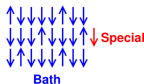
Our first example consists of the system shown in figure 23.1. The system is divided into two subsystems: Subsystem “B” is shown in blue, and will sometimes serve as “bath” (i.e. heat bath). Subsystem “S” is shown in scarlet, and will sometimes be referred to as the “small” or “special” subsystem.
In general there are NS sites in the scarlet subsystem, NB sites in the blue subsystem, for a total of N=NS+NB sites overall. We start by considering the case where NS=1, NB=1000, and N=1001.
For clarity, there are only NB=24 blue sites shown in the figure, so you will have to use your imagination to extrapolate to NB=1000.
The overall system B+S is isolated so that its energy is constant. The various sites within the overall system are weakly interacting, so that they can exchange energy with each other. In our first example, all N sites in the overall system are equivalent. That is, we have arbitrarily designated one of the sites as “special” but this designation has no effect on the physics of the overall system.
Each of the N sites can be in one of two states, either up or down. The energy of the up state is higher than the energy of the down state by one unit.
We have arranged that m of the N sites are in the up state. We choose the zero of energy such that E=m. We shall be particularly interested in the case where m=250 and N=1001.
The overall system has only one macrostate, namely the set of all microstates consistent with the given (constant) values of total N and total energy E. There are W microstates in the given macrostate, where W is called the multiplicity.
Figure 23.1 is a snapshot, showing only one microstate of the overall system. By conservation of energy we have constant m, so we can find all the other microstates by simply finding all permutations, i.e. all ways of assigning m up labels to N sites. That means the multiplicity can be computed in terms of the binomial coefficient:
| (23.3) |
|
For the present example, the numerical values are:
| (23.4) |
The microstates are all equivalent, so the probability of the ith microstate is Pi = 1/W for all i.
Let’s think about the symmetry of the situation. All N sites are equivalent, so we expect that anything that happens at one site is equally likely to happen at any other site.
Because (by construction) m is very nearly one fourth of N, if we pick any site at random, it is very nearly three times as likely to be in the down state as in the up state. Since we imagine that the sites are freely exchanging energy, we can replace the average over sites by a time average at a single site, whereupon we see that the scarlet site (or any other site) is three times as likely to be found in the down state as in the up state. In symbols:
| (23.5) |
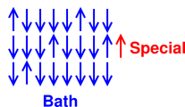
We can define two categories of microstates: one where the special site is in the down state (which we call x=0, as in figure 23.1), and another where the special site is in the up state (which we call x=1, as in figure 23.2).
These categories are in some ways just like macrostates, in the sense that they are sets of microstates. However, for clarity we choose to call them categories not macrostates. We can calculate the multiplicity of each category separately. As before, all we need to do is count permutations. Within each category, however, we only consider permutations of the blue sites because the state of the scarlet site is fixed.
We can streamline the discussion by borrowing some notation that is commonly applied to chemical reactions. Here x is the reaction coordinate. The reaction of interest involves the transfer of one unit of energy to the special site from the heat bath. That is:
| (23.6) |
The multiplicity of the x=1 category is less, because when we do the permutations, there is one fewer “up” state to play with.
Whether or not we assign these microstates to categories, they are still microstates of the overall system. Therefore they all have the same energy, since the system is isolated. Therefore the microstates are all equally probable, in accordance with proposition (1) as set forth at the beginning of section 23.1.
If you look at the numbers in equation 23.6, you see that the x=0 microstates are very nearly threefold more numerous than the x=1 microstates. We can calculate this exactly in terms of m and N:
| (23.7) |
You can verify algebraically that the ratio of multiplicities is exactly equal to m/(N−m). This factor shows up in both equation 23.5 and equation 23.7, which means the probability we get by counting microstates is provably identical to the probability we get from symmetry arguments.
Consistency is always nice, but in this case it doesn’t tell us much beyond what we already knew. (Things will get much more exciting in a moment.)
Feel free to skip the following tangential remark. It is just another consistency check. The rest of the development does not depend on it.Let’s check that the multiplicity values for the categories are consistent with the multiplicity of the overall system.
Each category has a certain multiplicity. If we add these two numbers together, the sum should equal the multiplicity of the overall system.
We know this “should” be true, because we have exhausted all the possibilities.
We can verify that it is in fact true by using the mathematical properties of the binomial coefficients, especially the fact that each entry in Pascal’s triangle is the sum of the two entries above it on the previous row. To say the same thing more formally, you can easily verify the following algebraic identity:
⎛
⎜
⎝
N m ⎞
⎟
⎠=
⎛
⎜
⎝
N−1 m ⎞
⎟
⎠+
⎛
⎜
⎝
N−1 m−1 ⎞
⎟
⎠(23.8)
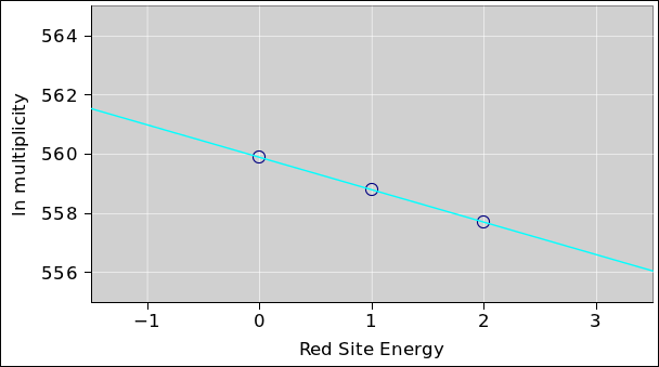
To obtain a clearer picture of what is going on, and to obtain a much stricter check on the correctness of what we have done, we now increase the number of scarlet sites to NS=2. To keep things simple we increase the total N to 1002 and increase m to 251. The reaction coordinate can now take on the values x=0, x=1, and x=2. I’m not going to bother redrawing the pictures.
The trick of calculating the scarlet-subsystem probabilities by appeal to symmetry still works (although it isn’t guaranteed to work for more complicated systems). More importantly, we can always calculate the probability by looking at the microstates; that always works. Indeed, since the microstates of the overall system are equiprobable, all we need to do is count them.
| (23.9) |
The situation is shown in figure 23.3. We see that every time the scarlet subsystem energy goes up (additively), the bath energy goes down (additively), the multiplicity goes down (multiplicatively), and therefore the log multiplicity goes down (additively). Specifically, the log multiplicity is very nearly linear in the energy, as you can see from the fact that (to an excellent approximation) the points fall on a straight line in figure 23.3.
If we define temperature to be the negative reciprocal of the slope of this line, then this example upholds proposition (2). This definition is consistent with the previous definition, equation 7.7.
Our example is imperfect in the sense that the three points in figure 23.3 do not fall exactly on a straight line. Therefore our example does not exactly uphold proposition (2). On the other hand, it is quite a good approximation. The points fall so nearly on a straight line that you probably can’t see any discrepancy by looking at the figure. We shall demonstrate in a moment that there is some nonzero discrepancy. This is not tragic; we can rationalize it by saying that a bath consisting of 1000 sites is a slightly imperfect heat bath. In the limit as N and m go to infinity, the bath becomes perfect.
We can quantify the imperfection as follows: The probability ratio between the upper two points is:
| = |
| (23.10) |
Meanwhile, the ratio between the lower two points is:
| = |
| (23.11) |
which is obviously not the same number. On the other hand, if you pass to the limit of large N and large m, these two ratios converge as closely as you like. (Also note that these two ratios bracket the ratio given in equation 23.7.)
We have just seen that the advantages of having a heat bath with a large number of sites.
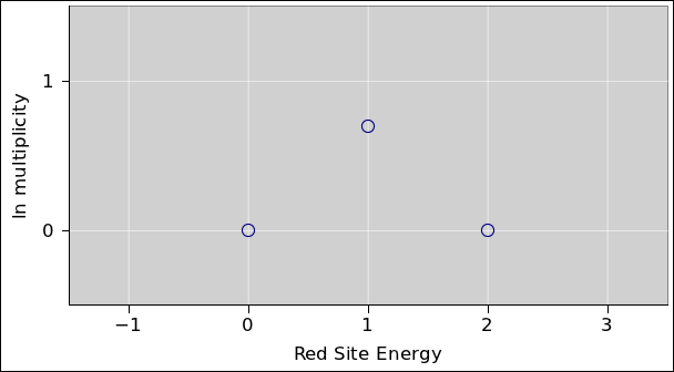
To emphasize this point, let’s see what happens when NB is small. In particular, consider the case where NB=2, NS=2, and m=2. Then the ratios in equation 23.10 and equation 23.11 are 2:1 and 1:2 respectively ... which are spectacularly different from each other. The situation is shown in figure 23.4.
Obviously these points do not lie on a straight line. The probabilities do not follow a Boltzmann distribution, not even approximately. A major part of the problem is that the blue subsystem, consisting of NB=2 sites, is not a good heat bath, not even approximately.
In this situation, temperature is undefined and undefinable, even though the system satisfies Feynman’s definition of thermal equilibrium, i.e. when all the fast things have happened and the slow things have not. This is the maximum entropy macrostate, the most entropy the system can have subject to the stipulated constraints (constant N and constant m). This is a very peculiar state, but as far as I can tell it deserves to be labeled the equilibrium state. Certainly there is no other state with a stronger claim to the label.
Note that the 1:2:1 ratio we are discussing, as shown in figure 23.4, gives the probability per microstate for each of the four microstates. If you are interested in the probability of the three energy levels, the answer is 1:4:1, because the x=1 energy level has twice the multiplicity of the others. Always remember that the probability of a macrostate depends on the number of microstates as well as the probability per microstate.
The situation shown in figure 23.4 may seem slightly contrived, since it applies to thermal equilibrium in the absence of any well-behaved heat bath. However, the same considerations sometimes come into play even when there is a heat bath involved, if we use it bath-backwards. In particular, we now return to the case where N=1002 and NS=2. We saw in section 23.3 that in this situation, the scarlet subsystem exhibits a Boltzmann distribution, in accordance with proposition (2). But what about the blue subsystem?
It turns out that each and every microstate of the blue subsystem in the x=0 and x=2 categories has the same probability, even though they do not all have the same energy. This means that the blue microstate probabilities do not follow a Boltzmann distribution.
Furthermore, each blue microstate in the x=1 category has twice as much probability as any x=0 or x=2 microstate, because there are two ways it can happen, based on the multiplicity of the corresponding microstates of the overall subsystem. That is, when x=1, there are two microstates of the overall system for each microstate of the blue subsystem (due to the multiplicity of the scarlet subsystem), and the microstates of the overall system are equiprobable. The result is closely analogous to the situation shown in figure 23.4.
The way to understand this is to recognize that when NS=2, the scarlet subsystem is too small to serve as a proper heat bath for the blue subsystem.
At this point, things are rather complicated. To help clarify the ideas, we rearrange the Boltzmann distribution law (equation 23.2) as follows:
| Tµ:= |
|
| (23.12) |
for any two microstates i and j. We take this as the definition of Tµ, where µ refers to microstate.
We contrast this with the conventional definition of temperature
| TM := |
|
| (23.13) |
We take this as the definition of TM, where M refers to macrostate. As far as I can tell, this TM is what most people mean by “the” temperature T. It more-or-less agrees with the classical definition given in equation 7.7.
It must be emphasized that when two subsystems are in contact, the Boltzmann property of one system depends on the bath-like behavior of the other. The Tµ of one subsystem is equal to the TM of the other. That is, S is Boltzmann-distributed if B is a well-behaved heat bath; meanwhile S is Boltzmann-distributed if B is a well-behaved heat bath.
To say the same thing the other way, you cannot think of a subsystem as serving as a bath for itself. In the present example, for the blue subsystem TM is well defined but Tµ is undefined and undefinable, while for the scarlet subsystem the reverse is true: Tµ is well defined but TM is undefined and undefinable.
Among other things, we have just disproved proposition (3).
If you think that is confusing, you can for homework consider the following situation, which is in some ways even more confusing. It serves to even more dramatically discredit the idea that two subsystems in equilibrium must have the same temperature.
We have just considered the case where the scarlet subsystem consisted of two spin-1/2 particles, so that it had four microstates and three energy levels. Now replace that by a single spin-1 particle, so that it has only three microstates (and three energy levels).
In this scenario, there are three macrostates of the blue subsystem, corresponding to three different energies. The odd thing is that each and every microstate of the blue subsystem has exactly the same probability, even though they do not all have the same energy.
In some perverse sense these blue microstates can be considered consistent with a Boltzmann distribution, if you take the inverse temperature β to be zero (i.e. infinite temperature).
This situation arises because each energy level of the scarlet system has the same multiplicity, WS = 1. Therefore the log multiplicity is zero, and β = (d/dE) ln(W) = 0.
This situation is mighty peculiar, because we have two subsystems in equilibrium with each other both of which are Boltzmann-distributed, but which do not have the same temperature. We are attributing an infinite temperature to one subsystem and a non-infinite temperature to the other. This can’t be good.
Note that in all previous scenarios we were able to calculate the probability in two different ways, by symmetry and by counting the microstates. However, in the present scenario, where we have a spin-1 particle in equilibrium with a bunch of spin-1/2 particles, we cannot use the symmetry argument. We can still count the microstates; that always works.
We can deepen our understanding by considering yet another example.
At each of the blue sites, we replace what was there with something where the energy splitting is only half a unit. Call these “light blue” sites if you want. Meanwhile, the scarlet sites are the same as before; their energy splitting remains one full unit.
In this situation, m is no longer a conserved quantity. Whenever the reaction coordinate x increases by one, it annihilates two units of mB and creates one unit of mS. Energy is of course still conserved: E = mS + mB/2.
We wish the scarlet subsystem to remain at the same temperature as in previous examples, which means we want its up/down ratio to remain at 1/3. To do this, we must drastically change the up/down ratio of the blue subsystem. Previously it was 1/3 but we shall see that now it must be √1/3.
In our numerical model, we represent this by NB=1000 and mB=368−2x.
Now, whenever we increase x by one, we now have two fewer up states to play with in the blue subsystem, so the multiplicity changes by two factors, each of which is very nearly mB/(NB−mB i.e. very nearly √3. The two factors together mean that the multiplicity changes by a factor of 3, which means the probability of the S microstates changes by a factor of 3, as desired.
One reason for working through the “light blue” scenario is to emphasize that the RHS of equation 23.13 is indeed properly written in terms of W and E ... in contrast to various other quantities that you might have thought would be more directly important.
There is a long list of things that might seem directly important, but are not. When two systems are in equilibrium:
The list of things that do matter is much shorter: When two subsystems are in thermal equilibrium:
These points are particularly clear in the “light blue” scenario (section 23.6). When setting up the problem, we needed to supply “just enough” energy to achieve the desired temperature, i.e. the desired TM, i.e. the desired Δln(W)/ΔE. The amount of energy required to do this, 183 units, might not have been obvious a priori.
Suppose you have one heat bath in contact with another.
If they start out at different temperatures, energy will flow from one to the other. This will continue until the TM of one lines up with the Δln(W)/ΔE of the other.
This depends on ln(W) being a convex function of E. This is not an entirely trivial assumption. For one thing, it means that in two dimensions, a single particle in a box would not be a good heat bath, since its density of states is independent of E. Multiple particles in a box works fine, even in two dimensions, because the combinatorial factors come to the rescue.
Sometimes it is suggested that the discrepancies and limitations discussed in this chapter are irrelevant, because they go away in the large-N limit, and thermodynamics only applies in the large-N limit.
Well, they do go away in the large-N limit, but that does not make them irrelevant. Vast parts of thermodynamics do make sense even for small-N systems. It is therefore important to know which parts we can rely on and which parts break down when stressed. Important small-N applications include reversible computing and quantum computing. Also, the standard textbook derivation of the Boltzmann factor uses a small-NS argument. If we are going to make such an argument, we ought to do it correctly.