Terminology: By definition, the term state function applies to any measurable quantity that is uniquely determined by the thermodynamic state, i.e. the macrostate.
Terminology: The term thermodynamic potential is synonymous with state function. Also the term function of state is synonymous with state function.
Example: In an ordinary chunk of metal at equilibrium, state functions include energy (E), entropy (S), temperature (T), molar volume (V/N), total mass, speed of sound, et cetera. Some additional important thermodynamic potentials are discussed in chapter 15.
In thermodynamics, we usually arrange for the energy E to be a function of state. This doesn’t tell us anything about E, but it tells us something about our notion of thermodynamic state. That is, we choose our notion of “state” so that E will be a function of state.
Similarly, we usually arrange for the entropy S to be a function of state.
When identifying functions of state, we make no distinction between dependent variables and independent variables. For example, suppose you decide to classify V and T as independent variables. That doesn’t disqualify them from being functions of state. Calculating V as a function of V and T is not a hard problem. Similarly, calculating T as a function of V and T is not a hard problem. I wish all my problems were so easy.
Counterexample: The microstate is not a function of state (except in rare extreme cases). Knowing the macrostate is not sufficient to tell you the microstate (except in rare extreme cases).
Counterexample: Suppose we have a system containing a constant amount H2O. Under “most” conditions, specifying the pressure and temperature suffices to specify the thermodynamic state. However, things get ugly if the temperature is equal to the freezing temperature (at the given pressure). Then you don’t know how much of the sample is liquid and how much is solid. In such a situation, pressure and temperature do not suffice to specify the thermodynamic state. (In contrast, specifying the pressure and entropy would suffice.)
Note that to be a state function, it has to be a function of the macrostate. This is an idomatic usage of the word “state”.
Something that is a function of the macrostate might or might not make sense as a function of the microstate. Here are some contrasting examples:
| The energy is a function of the macrostate, and also a well-behaved function of the microstate. The same can be said for some other quantities including mass, volume, charge, chemical composition, et cetera. | The entropy is a function of the macrostate, but not a function of the microstate. It is defined as an ensemble average. If the macrostate consists of a single microstate, its entropy is zero. |
A crucial prerequisite to idea of “state function” is the idea of “thermodynamic state” i.e. macrostate. Thermodynamics is predicated on the idea that the macrostate can be described by a few variables, such as P, V, T et cetera. This stands in contrast to describing the microstate, which would require something like 1023 variables.
In fluid dynamics, we might divide the fluid into a thousand parcels, each with its own state functions Pi, Vi, Ti et cetera. That means we have thousands of variables, but that’s still a small number compared to 1023.
Functions of state can be well defined even if the system as a whole is not in equilibrium. For example, the earth’s troposphere is nowhere near thermal equilibrium. (In equilibrium, it would be isothermal, for reasons discussed in section 14.4.) In such a situation, we divide the system into parcels. As long as the parcel unto itself has a well-defined temperature, we can consider temperature to be a function of state, i.e. a function of the state of that parcel.
When we say that something is a function of state, we are saying that it does not depend on history; it does not depend on how we got into the given state.
We can apply this idea to changes in any function of state. For example, since E is a function of state, we can write
| (7.1) |
When we say that ΔE is independent of path, that mean that ΔE is the same, no matter how many steps it takes to get from the initial state to the final state. The path can be simple and direct, or it can involve all sorts of loops and cycles.
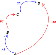
As a corollary, if we get from state A to state D by two different paths, as shown in figure 7.1, if we add up the changes along each step of each paths, we find that the sum of the changes is independent of paths. That is,
| ΔAD(X) = ΔAB(X) + ΔBC(X) + ΔCD(X) (7.2) |
As usual Δ(X) refers to the change in X. Here X can any thermodynamic potential.
The term sigma-delta is sometimes used to refer to a sum of changes. Equation 7.2 states that the sigma-delta is independent of path.
It must be emphasized that the principle of the path-independent sigma-delta has got nothing to do with any conservation law. It applies to non-conserved state-functions such as temperature and molar volume just as well as it applies to conserved state-functions such as energy. For example, if the volume V is a function of state, then:
| (7.3) |
which is true even though V is obviously not a conserved quantity.
Equation 7.3 looks trivial and usually is trivial. That’s because usually you can easily determine the volume of a system, so it’s obvious that ΔV is independent of path.
The derivation of equation 7.1 is just as trivial as the derivation of equation 7.3, but the applications of equation 7.1 are not entirely trivial. That’s because you can’t always determine the energy of a system just by looking at it. It may be useful to calculate ΔE along one simple path, and then argue that it must be the same along any other path connecting the given initial and final states.
Remark: It is a fairly common mistake for people to say that ΔE is a function of state. It’s not a function of state; it’s a function of two states, namely the initial state and the final state, as you can see from the definition: ΔE = Efinal − Einitial. For more on this, see reference 4. As explained there,
- ΔE is a scalar but not a function of state.
- dE is a function of state but not a scalar.
Circa 1840, Germain Henri Hess empirically discovered a sum rule for the so-called heat of reaction. This is called Hess’s Law. Beware that it is not always true, because the heat of reaction is not a function of state.
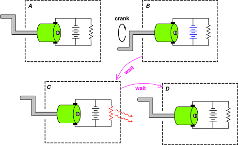
A simple counterexample is presented in figure 7.2.
We start in the upper left of the figure. We turn the crank on the generator, which charges the battery. That is, electrochemical reactions take place in the battery. We observe that very little heat is involved in this process. The charged-up battery is shown in blue.
If we stop cranking and wait a while, we notice that this battery has a terrible shelf life. Chemical reactions take place inside the battery that discharge it. This is represented conceptually by a “leakage resistor” internal to the battery. This is represented schematically by an explicit resistor in figure 7.2. In any event, we observe that the battery soon becomes discharged, and becomes warmer. If we wait a little longer, heat flows across the boundary of the system (as shown by the wavy red arrows). Eventually we reach the state shown in the lower right of the diagram, which is identical to the initial state.
There is of course a simpler path for reaching this final state, namely starting at the same initial state and doing nothing ... no cranking, and not even any waiting. This clearly violates Hess’s law because the heat of reaction of the discharge process is the dominant contribution along one path, and nothing similar is observed along the other path.
Hess’s law in its original form is invalid because heat content is not a state function, and heat of reaction is not the delta of any state function.
Tangential remark: in cramped thermodynamics, a cramped version of Hess’s Law is usually valid, because “heat content” is usually a function of state in cramped thermodynamics. This is a trap for the unwary. This is just one of the many things that are true in cramped thermodynamics but cannot be extended to uncramped thermodynamics.
We can extricate ourselves from this mess by talking about enthalpy instead of heat. There is a valid sum rule for the enthalpy of reaction, because enthalpy is a function of state. That is:
| (7.4) |
We emphasize that this does not express conservation of enthalpy. In fact, enthalpy is not always conserved, but equation 7.4 remains true whenever enthalpy is a function of state.
Equation 7.4 could be considered a modernized, “repaired” version of Hess’s law. It is not very important. It does not tell us anything about the enthalpy except that it is a function of state. It is a mistake to focus on applying the sigma-delta idea to enthalpy to the exclusion of the innumerable other state-functions to which the sigma-delta idea applies equally well.
I see no value in learning or teaching any version of Hess’s Law. It is better to simply remember that there is a sigma-delta law for any function of state.
Let’s build up a scenario, based on some universal facts plus some scenario-specific assumptions.
We know that the energy of the system is well defined. Similarly we know the entropy of the system is well defined. These aren’t assumptions. Every system has energy and entropy.
Next, as mentioned in section 7.1, we assume that the system has a well-defined thermodynamic state, i.e. macrostate. This macrostate can be represented as a point in some abstract state-space. At each point in macrostate-space, the macroscopic quantities we are interested in (energy, entropy, pressure, volume, temperature, etc.) take on well-defined values.
We further assume that this macrostate-space has dimensionality M, and that M is not very large. (This M may be larger or smaller than the dimensionality D of the position-space we live in, namely D=3.)
Assuming a well-behaved thermodynamic state is a highly nontrivial assumption.
We further assume that the quantities of interest vary smoothly from place to place in macrostate-space.
We must be careful how we formalize this “smoothness” idea. By way of analogy, consider a point moving along a great-circle path on a sphere. This path is nice and smooth, by which we mean differentiable. We can get into trouble if we try to describe this path in terms of latitude and longitude, because the coordinate system is singular at the poles. This is a problem with the coordinate system, not with the path itself. To repeat: a great-circle route that passes over the pole is differentiable, but its representation in spherical polar coordinates is not differentiable.Applying this idea to thermodynamics, consider an ice/water mixture at constant pressure. The temperature is a smooth function of the energy content, whereas the energy-content is not a smooth function of temperature. I recommend thinking in terms of an abstract point moving in macrostate-space. Both T and E are well-behaved functions, with definite values at each point in macrostate-space. We get into trouble if we try to parameterize this point using T as one of the coordinates, but this is a problem with the coordinate representation, not with the abstract space itself.
We will now choose a particular set of variables as a basis for specifying points in macrostate-space. We will use this set for a while, but we are not wedded to it. As one of our variables, we choose S, the entropy. The remaining variables we will collectively call V, which is a vector with D−1 dimensions. In particular, we choose the macroscopic variable V in such a way that the microscopic energy Êi of the ith microstate is determined by V. (For an ideal gas in a box, V is just the volume of the box.)
Given these rather restrictive assumptions, we can write:
| dE = |
| ⎪ ⎪ ⎪ ⎪ |
| dV + |
| ⎪ ⎪ ⎪ ⎪ |
| dS (7.5) |
which is just the chain rule for differentiating a function of two variables. Important generalizations of this equation can be found in section 7.6 and section 18.1.
It is conventional to define the symbols
| P := − |
| ⎪ ⎪ ⎪ ⎪ |
| (7.6) |
and
| (7.7) |
You might say this is just terminology, just a definition of T … but we need to be careful because there are also other definitions of T floating around. For starters, you can compare equation 7.7 with equation 15.11. More importantly, we need to connect this definition of T to the real physics, and to operational definitions of temperature. There are some basic qualitative properties that temperature should have, as discussed in section 11.1, and we need to show that our definition exhibits these properties. See chapter 13.
Equation 7.7 is certainly not the most general definition of temperature, because of several assumptions that we made in the lead-up to equation 7.5. By way of counterexample, in NMR or ESR, a τ2 process changes the entropy without changing the energy. As an even simpler counterexample, internal leakage currents within a thermally-isolated storage battery increase the entropy of the system without changing the energy; see figure 1.3 and section 11.5.5.
Using the symbols we have just defined, we can rewrite equation 7.5 in the following widely-used form:
| (7.8) |
Again: see equation 7.33, equation 7.34, and section 18.1 for important generalizations of this equation.
Continuing down this road, we can rewrite equation 7.8 as
| dE = w + q (7.9) |
where we choose to define w and q as:
| (7.10) |
and
| (7.11) |
That’s all fine; it’s just terminology. Note that w and q are one-forms, not scalars, as discussed in section 8.2. They are functions of state, i.e. uniquely determined by the thermodynamic state.1
Equation 7.9 is fine so long as we don’t misinterpret it. However, beware that equation 7.9 and its precursors are very commonly misinterpreted. In particular, it is tempting to interpret w as “work” and q as “heat”, which is either a good idea or a bad idea, depending on which of the various mutually-inconsistent definitions of “work” and “heat” you happen to use. See section 17.1 and section 18.1 for details.
Also: Equation 7.8 is sometimes called the “thermodynamic identity” although that seems like a bit of a misnomer. The only identity involved comes from calculus, not from thermodynamics. We are using a calculus identity to expand the exterior derivative dE in terms of some thermodynamically-interesting variables.
Beware that equation 7.8 has got little or nothing to do with the first law of thermodynamics, i.e. with conservation of energy. It has more to do with the fact that E is a differentiable function of state than the fact that it is conserved. None of the steps used to derive equation 7.8 used the fact that E is conserved. You could perhaps connect this equation to conservation of energy, but you would have to do a bunch of extra work and bring in a bunch of additional information, including things like the third law of motion, et cetera. To appreciate what I’m saying, it may help to apply the same calculus identity to some non-conserved function of state, perhaps the Helmholtz free energy F. You can go through the same steps and get an equation that is very similar to equation 7.8, as you can see in figure 15.10. If you did not already know what’s conserved and what not, you could not figure it out just by glancing at the structure of these equations.
Here’s another change of variable that calls attention to some particularly interesting partial derivatives. Now that we have introduced the T variable, we can write
| dE = |
| ⎪ ⎪ ⎪ ⎪ |
| dV + |
| ⎪ ⎪ ⎪ ⎪ |
| dT (7.12) |
assuming things are sufficiently differentiable.
The derivative in the second term on the RHS is conventionally called the heat capacity at constant volume. As we shall see in connection with equation 7.19, it is safer to think of this as the energy capacity. The definition is:
| CV := |
| ⎪ ⎪ ⎪ ⎪ |
| (7.13) |
again assuming the RHS exists. (This is a nontrivial assumption. By way of counterexample, the RHS does not exist near a first-order phase transition such as the ice/water transition, because the energy is not differentiable with respect to temperature there. This corresponds roughly to an infinite energy capacity, but it takes some care and some sophistication to quantify what this means. See reference 19.)
The energy capacity in equation 7.13 is an extensive quantity. The corresponding intensive quantities are the specific energy capacity (energy capacity per unit mass) and the molar energy capacity (energy capacity per particle).
The other derivative on the RHS of equation 7.12 doesn’t have a name so far as I know. It is identically zero for a table-top sample of ideal gas (but not in general).
The term isochoric means “at constant volume”, so CV is the isochoric heat capacity ... but more commonly it is just called the “heat capacity at constant volume”.
Using the chain rule, we can find a useful expression for CV in terms of entropy:
| (7.14) |
This equation is particularly useful in reverse, as means for measuring changes in entropy. That is, if you know CV as a function of temperature, you can divide it by T and integrate with respect to T along a contour of constant volume. The relevant formula is:
| (7.15) |
We could have obtained the same result more directly using the often-important fact, from equation 7.8,
| (7.16) |
and combining it with the definition of CV from equation 7.12 and equation 7.13:
| (7.17) |
Equation 7.17 is useful, but there are some pitfalls to beware of. For a given sample, you might think you could ascertain the absolute entropy S at a given temperature T by integrating from absolute zero up to T. Alas nobody has ever achieved absolute zero in practice, and using an approximation of zero K does not necessarily produce a good approximation of the total entropy. There might be a lot of entropy hiding in that last little interval of temperature. Even in theory this procedure is not to be trusted. There are some contributions to the entropy – such as the entropy of mixing – that may be hard to account for in terms of dS = dE/T. Certainly it would disastrous to try to “define” entropy in terms of dS = dE/T or anything like that.
Remark: Equation 7.12 expands the energy in terms of one set of variables, while equation 7.5 expands it in terms of another set of variables. This should suffice to dispel the misconception that E (or any other thermodynamic potential) is “naturally” a function of one set of variables to the exclusion of other variables. See section 15.7 and reference 3 for more on this.
This concludes our discussion of the constant-volume situation. We now turn our attention to the constant-pressure situation.
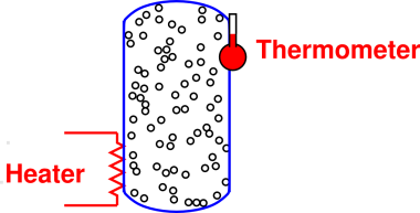
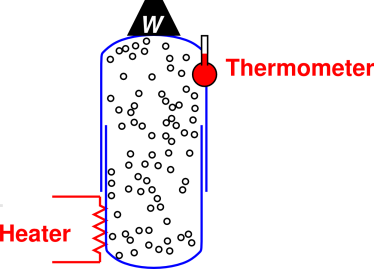
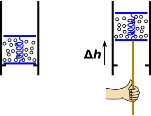
Operationally, it is often easier maintain constant ambient pressure than to maintain constant volume. For a gas or liquid, we can measure some sort of “heat capacity” using an apparatus along the lines shown in figure 7.4. That is, we measure the temperature of the sample as a function of the energy put in via the heater. However, this energy is emphatically not the total energy crossing the boundary, because we have not yet accounted for the PdV work done by the piston as it moves upward (as it must, to maintain constant pressure), doing work against gravity via the weight W. Therefore the energy of the heater does not measure the change of the real energy E of the system, but rather of the enthalpy H, as defined by equation 15.5.
This experiment can be modeled using the equation:
| dH = |
| ⎪ ⎪ ⎪ ⎪ |
| dP + |
| ⎪ ⎪ ⎪ ⎪ |
| dT (7.18) |
This is analogous to equation 7.12 ... except that we emphasize that it involves the enthalpy instead of the energy. The second term on the right is conventionally called the heat capacity at constant pressure. It is however safer to call it the enthalpy capacity. The definition is:
| CP := |
| ⎪ ⎪ ⎪ ⎪ |
| (7.19) |
Under favorable conditions, the apparatus for measuring CV for a chunk of solid substance is particularly simple, because don’t need the container and piston shown in figure 7.4; the substance contains itself. We just need to supply thermal insulation. The analysis of the experiment remains the same; in particular we still need to account for the PdV work done when the sample expands, doing work against the ambient pressure.
The term isobaric means “at constant pressure”, so another name for CP is the isobaric heat capacity.
In analogy to equation 7.15 we can write
| (7.20) |
which we can obtain using the often-important fact, from equation 15.6,
| (7.21) |
and combining it with the definition of CP from equation 7.18 and equation 7.19:
| (7.22) |
Collecting results for comparison, we have
| (7.23) |
Remark: We see once again that the term “heat” is ambiguous in ways that entropy is not. In the first two rows, the LHS is different, yet both are called “heat”, which seems unwise. In the second two rows, the LHS is the same, and both are called entropy, which is just fine.
Starting with either of the last two lines of equation 7.23 and solving for the heat capacity, we see that we can define a generalized heat capacity as:
| (7.24) |
where X can be just about anything, including X≡V or X≡P.
Remark: Heat capacity has the same dimensions as entropy.
We see from equation 7.24 that the so-called heat capacity can be thought of as the entropy capacity ... especially if you use a logarithmic temperature scale.
Equation 7.24 is useful for many theoretical and analytical purposes, but it does not directly correspond to the way heat capacities are usually measured in practice. The usual procedure is to observe the temperature as a function of energy or enthalpy, and to apply equation 7.13 or equation 7.19.
This supports the point made in section 0.3 and section 17.1, namely that the concept of “heat” is a confusing chimera. It’s part energy and part entropy. It is neither necessary nor possible to have an unambiguous understanding of “heat”. If you understand energy and entropy, you don’t need to worry about heat.
In section 7.4 we temporarily assumed that the energy is known as a function of entropy and volume. This is certainly not the general case. We are not wedded to using V and S as coordinates for mapping out the thermodynamic state space (macrostate space).
The point of this section is not to make your life more complicated by presenting lots of additional equations. Instead, the main point is to focus attention on the one thing that really matters, namely conservation of energy. The secondary point is that equations such as equation 7.8, equation 7.27, et cetera fall into a pattern: they express the exterior derivative of E in terms of the relevant variables, relevant to this-or-that special situation. Once you see the pattern, you realize that the equations are not at all fundamental.
Here is a simple generalization that requires a bit of thought. Suppose we have a parcel of fluid with some volume and some entropy. You might think we could write the energy as a function of V and S, as in equation 7.25 but that is not always sufficient, as we shall soon see.
| (7.25) |
Consider the apparatus shown in figure 7.5. The parcel of fluid is trapped between two pistons in the same cylinder. On the left is the initial situation.
On the right we see that the parcel has been raised by a distance Δh. It was raised slowly, gently, and reversibly, using a thermally-insulating pushrod. The entropy of the parcel did not change. The volume of the parcel did not change. Overall, no work was done on the parcel.
The interesting thing is that the gravitational potential energy of the parcel did change.
Nitpickers may argue about whether the gravitational energy is “in” the parcel or “in” the gravitational field, but we don’t care. In any case, the energy is associated with the parcel, and we choose to include it in our definition of E, the energy “of” the parcel. The idea of E = m g h is perhaps the first and most basic energy-related formula that you ever saw.
The exterior derivative must include terms for each of the relevant variables:
| (7.26) |
Under mild conditions this simplifies to:
| (7.27) | |||||||||||||||||||||||
where m g is the weight of the parcel. There are two “mechanical” terms.
Equation 7.27 tells us that we can change the energy of the parcel without doing work on it. This should not come as a surprise; there is a work/kinetic-energy theorem, not a work/total-energy theorem.
Nevertheless this does come as a surprise to some people. Part of the problem is that sometimes people call equation 7.8 “the” first law of thermodynamics. They treat it as “the” fundamental equation, as if it were the 11th commandment. This leads people to think that the only way of changing the energy of the parcel is by doing mechanical work via the P dV term and/or exchanging heat via the T dS term. Let’s be clear: the m g dh term is mechanical, but it is not work (not P dV work, and not overall work from the parcel’s point of view).
Another part of the problem is that when thinking about thermodynamics, people sometimes think in terms of an oversimplified model system, perhaps a small (“table-top”) sample of ideal gas. They make assumptions on this basis. They equate “mechanical energy transfer” with work. Then, when they try to apply their ideas to the real world, everything goes haywire. For a table-top sample of ideal gas, moving it vertically makes only a small contribution to the energy, negligible in comparison to ordinary changes in pressure or temperature. However, the contribution is not small if you’re looking at a tall column of air in the earth’s atmosphere, or water in the ocean, or the plasma in the sun’s atmosphere, et cetera. Vertical motions can have tremendous implications for temperature, pressure, stability, transport, mixing, et cetera.
A liquid is typically 1000 times denser than a gas at STP. So if you imagine the fluid in figure 7.5 to be a liquid rather than a gas, the m g dh contribution is 1000 times larger.
In a situation where we know the volume is constant, equation 7.27 simplifies to:
| (7.28) |
That superficially looks like equation 7.8 (with an uninteresting minus sign). On the RHS we can identify a “thermal” term and a “mechanical” term. However, it is spectacularly different for a non-obvious reason. The reason is that V and h enter the equation of state in different ways. Changing V at constant h and S changes the temperature and pressure, whereas changing h at constant V and S does not. For the next level of detail on this, see section 9.3.4.
Some folks try to simplify equation 7.27 by rewriting it in terms of the «internal energy», but I’ve never found this to be worth the trouble. See section 7.7.
Here’s a simple but useful reformulation. It doesn’t involve any new or exciting physics. It’s the same idea as in section 7.4, just with slightly different variables: forces instead of pressure.
Suppose we have a box-shaped parcel of fluid. As it flows along, it might change its size in the X direction, the Y direction, or the Z direction. The volume is V = XYZ. Instead of equation 7.5 we write:
| (7.29) |
where we define the force FX as a directional derivative of the energy:
| (7.30) |
and similarly for the forces in the Y and Z directions. Compare equation 18.5.
Here’s another widely-useful generalization. Sometimes we have a box where the number of particles is not constant. We might be pumping in new particles and/or letting old particles escape. The energy will depend on the number of particles (N). The exterior derivative is then:
| dE = |
| ⎪ ⎪ ⎪ ⎪ |
| dN + |
| ⎪ ⎪ ⎪ ⎪ |
| dV + |
| ⎪ ⎪ ⎪ ⎪ |
| dS (7.31) |
For present purposes, we assume there is only one species of particles, not a mixture.
This is a more-general expression; now equation 7.5 can be seen a corollary valid in the special case where N is constant (so dN=0).
The conventional pet name for the first derivative on the RHS is chemical potential, denoted µ. That is:
| µ := |
| ⎪ ⎪ ⎪ ⎪ |
| (7.32) |
where N is the number of particles in the system (or subsystem) of interest.
This means we can write:
| dE = µ dN − P dV + T dS (7.33) |
which is a generalization of equation 7.8.
It is emphatically not mandatory to express E as a function of (V,S) or (N,V,S). Almost any variables that span the state-space will do, as mentioned in section 15.7 and reference 3.
You should not read too much into the name “chemical” potential. There is not any requirement nor even any connotation that there be any chemical reactions going on.
The defining property of the chemical potential (µ) is that it is conjugate to an increase in number (dN) … just as the pressure (P) is conjugate to a decrease in volume (−dV). Note the contrast: in the scenario described by equation 7.33:
| Stepping across a contour of −dV increases the density (same number in a smaller volume). | Stepping across a contour of dN increases the density (bigger number in the same volume). |
| This can happen if a piston is used to change the volume. | This can happen if particles are carried across the boundary of the system, or if particles are produced within the interior of the system (by splitting dimers or whatever). |
So we see that dN and dV are two different directions in parameter space. Conceptually and mathematically, we have no basis for declaring them to be “wildly” different directions or only “slightly” different directions; all that matters is that they be different i.e. linearly independent. At the end of the day, we need a sufficient number of linearly independent variables, sufficient to span the parameter space.
Equation 7.33 is a generalization of equation 7.8, but it is not the absolute most-general equation. In fact there is no such thing as the most-general equation; there’s always another generalization you can make. For example, equation 7.33 describes only one species of particle; if there is another species, you will have to define a new variable N2 to describe it, and add another term involving dN2 to the RHS of equation 7.33. Each species will have its own chemical potential. Similarly, if there are significant magnetic interactions, you need to define a variable describing the magnetic field, and add the appropriate term on the RHS of equation 7.33. If you understand the meaning of the equation, such generalizations are routine and straightforward. Again: At the end of the day, any expansion of dE needs a sufficient number of linearly independent variables, sufficient to span the relevant parameter space.
For a more formal discussion of using the chain rule to expand differentials in terms of an arbitrary number of variables, see reference 3.
In general, we need even more variables. For example, for a parcel of fluid in a flow reactor, we might have:
| dE = ∑ µi dNi− P dV + m g dh + m v · dv+ T dS + ⋯ (7.34) |
where Ni is the number of molecular entities of the ith kind, m is the mass of the parcel, g is the acceleration of gravity, h is the height, v is the velocity, and the ellipsis (⋯) represents all the terms that have been left out.
Note that in many cases it is traditional to leave out the ellipsis, recognizing that no equation is fully general, and equation 7.33 is merely a corollary of some unstated cosmic generality, valid under the proviso that the omitted terms are unimportant.
Opinions differ, but one common interpretation of equation 7.34 is as follows: the TdS term can be called the “heat” term, the two terms − P dV + m g dh can be called “work” terms, the µi dNi is neither heat nor work, and I don’t know what to call the m v·dv term. Obviously the m v·dv term is important for fluid dynamics, and the µ dN term is important for chemistry, so you would risk getting lots of wrong answers if you rashly assumed equation 7.8 were “the” definition of heat and work.
As foreshadowed in section 1.8.4, a great many thermodynamics books emphasize the so-called «internal energy», denoted U or Ein. Mostly they restrict attention to situations where the «internal energy» is identically equal to the plain old energy, so I have to wonder why the bothered to introduce a fancy new concept if they’re not going to use it. In situations where the two concepts are not equivalent, things are even more mysterious. I have never found it necessary to make sense of this. Instead I reformulate everything in terms of the plain old energy E and proceed from there.
Feel free to skip this section ... but if you’re curious, the «internal energy» is defined as follows:
Suppose we have a smallish parcel of fluid with total mass M and total momentum Π as measured in the lab frame.2 Its center of mass is located at position R in the lab frame. Then we can express the «internal energy» of the parcel as:
| (7.35) |
where Φ is some potential. If it is a gravitational potential then Φ(R) = − M g·R, where g is a downward-pointing vector.
The «internal energy» is a function of state. As you can see from equation 7.35:
In other words, the «internal energy» can be thought of as the energy of a parcel as observed in a frame that is comoving with and colocated with the parcel’s center of mass. This can be considered a separation of variables. A complete description of the system can be thought of in terms of the variables in the center-of-mass frame plus the “special” variables that describe the location and velocity of the center-of-mass itself (relative to whatever frame we are actually using).
I’ve always found it easier to ignore the «internal energy» and use the plain old energy (E) instead, for multiple reasons:
| One parcel expands in such a way as to compress a neighboring parcel. Ein is conserved in this special case. So far so good. | One parcel expands in such a way as to hoist a neighboring parcel. It seems to me that Ein is not conserved. |
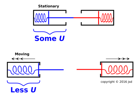
An even better argument that leads to the same conclusion is based on the situation shown in figure 7.6. There are two jack-in-the-box mechanisms. We focus attention on the blue one, on the left side of the diagram.
If you want to make this look more classically thermodynamical, you can replace each spring by some gas molecules under pressure. The idea is the same either way.
It should be obvious by symmetry that no energy crossed the boundary of the blue system. (Some momentum crossed the boundary, but that’s the answer to a different question.) No work was done by (or on) the blue system. There was no F·dx. The pushrod does not move until after contact has ceased and there is no longer any force. At the time and place where there was a nonzero force, there was no displacement. At times and places where there was a nonzero displacement, there was no force.
As a secondary argument leading to the same conclusion, you could equally well replace the red box by a rigid infinitely-massive wall. This version has fewer moving parts but less symmetry. Once again the displacement at the point of contact is zero. Therefore the F·dx work is zero. The pseudowork is nonzero, but the actual thermodynamic work is zero. (Pseudowork is discussed in section 18.5 and reference 18.)
The purpose of this Gedankenexperiment is to make a point about conservation and non-conservation:
| The plain old energy E is conserved. Some energy that was stored in the spring has been converted to KE ... more specifically, converted to KE associated with motion of the center of mass. | The «internal energy» is not conserved. The stored energy counts toward Ein, whereas the center-of-mass KE does not. |
It is widely believed3 that «if no matter or energy crosses the boundary of the system, then the internal energy is constant». First of all, this is not true, as demonstrated by figure 7.6. We can cook up a similar-sounding statement that is actually true, if we define a notion of super-isolated system, which cannot exchange matter, energy, momentum, or anything else. Still, even the repaired statement is highly misleading. It is practically begging people to reason by analogy to the plain old energy, which leads to the wrong answer about conservation of «internal energy», as we see from the following table:
Constant in a Conserved super-isolated system Energy : yes yes «Internal Energy» : yes no ← surprise! Table 7.1: Constancy versus Conservation
Just because some variable is constant in a super-isolated system does not mean it is conserved. There are plenty of counterexamples. In special relativity, mass is in this category, as discussed in reference 7. See section 1.2 and reference 6 for a discussion of what we mean by conservation.
The books that glorify Ein (aka U) typically write something like
| (7.36) |
and then assert that it expresses conservation of energy. I find this very odd, given that in reality U is not conserved.
Suggestion: If you are ever tempted to formulate thermodynamics in terms of «internal energy», start by calculating the heat capacity of a ten-mile-high column of air in a standard gravitational field. Hint: As you heat the air, its center of mass goes up, changing the gravitational potential energy, even though the container has not moved. I predict this will make you much less enamored of U, much less ready to enshrine it as the central focus of thermodynamics.
Here’s how I think about it: Very often there are some degrees of freedom that do not equilibrate with others on the timescale of interest. For example:
These special modes contribute to the energy in the usual way, even though they do not equilibrate in the usual way. It is necessary to identify them and assign them their own thermodynamic variables. On the other hand, as far as I can tell, it is not necessary or even helpful to define new «energy-like» thermodynamic potentials (such as Ein aka U).
Special variables yes; special potentials no. Note that the «internal energy» as usually defined gives special treatment to the center-of-mass kinetic energy but not to the battery electrical energy. That is yet another indicator that it doesn’t really capture the right idea.
Let’s continue to assume that T and P are functions of state, and that S and V suffice to span the macrostate-space. (This is certainly not always a safe assumption, as you can see in e.g. equation 7.27.)
Then, in cases where equation 7.8 is valid, we can integrate both sides to find E. This gives us an expression for E as a function of V and S alone (plus a constant of integration that has no physical significance). Naturally, this expression is more than sufficient to guarantee that E is a function of state.
Things are much messier if we try to integrate only one of the terms on the RHS of equation 7.8. Without loss of generality, let’s consider the T dS term. We integrate T dS along some path Γ. Let the endpoints of the path be A and B.
It is crucial to keep in mind that the value of the integral depends on the chosen path — not simply on the endpoints. It is OK to write things like
| sΔ QΓ = | ∫ |
| T dS (7.37) |
whereas it would be quite unacceptable to replace the path with its endpoints:
| (anything) = | ∫ |
| T dS (7.38) |
I recommend writing QΓ rather than Q, to keep the path-dependence completely explicit. This QΓ exists only along the low-dimensional subspace defined by the path Γ, and cannot be extended to cover the whole thermodynamic state-space. That’s because T dS is an ungrady one-form. See section 8.2 for more about this.
Equation 7.8 is predicated on the assumption that the energy is known as a function V and S alone. However, this is not the most general case. As an important generalization, consider the energy budget of a typical automobile. The most-common way of increasing the energy within the system is to transfer fuel (and oxidizer) across the boundary of the system. This is an example of advection of energy. This contributes to dE, but is not included in PdV or TdS. So we should write something like:
| dE = −P dV + T dS + advection (7.39) |
It is possible to quantify the advection mathematically. Simple cases are easy. The general case would lead us into a discussion of fluid dynamics, which is beyond the scope of this document.
Having derived results such as equation 7.8 and equation 7.39, we must figure out how to interpret the terms on the RHS. Please consider the following notions and decide which ones are true:
It turns out that these three notions are mutually contradictory. You have to get rid of one of them, for reasons detailed in section 17.1 and section 8.6.
As a rule, you are allowed to define your terms however you like. However, if you want a term to have a formal, well-defined meaning,
The problem is, many textbooks don’t play by the rules. On some pages they define heat to be TdS, on some pages they define it to be flow across a boundary, and on some pages they require thermodynamics to apply to irreversible processes.
This is an example of boundary/interior inconsistency, as discussed in section 8.6.
The result is a shell game, or a whack-a-mole game: There’s a serious problem, but nobody can pin down the location of the problem.
This results in endless confusion. Indeed, sometimes it results in holy war between the Little-Endians and the Big-Endians: Each side is 100% convinced that their definition is “right”, and therefore the other side must be “wrong”. (Reference 20.) I will not take sides in this holy war. Viable alternatives include:
For more on this, see the discussion near the end of section 7.11.
It is not necessarily wise to pick out certain laws and consider them “axioms” of physics. As Feynman has eloquently argued in reference 21, real life is not like high-school geometry, where you were given a handful of axioms and expected to deduce everything from that. In the real world, every fact is linked to many other facts in a grand tapestry. If a hole develops in the tapestry, you can re-weave it starting from the top of the hole, or the bottom, or either side. That is to say, if you forget one particular fact, you can re-derive it in many different ways.
In this spirit, some folks may wish to consider equation 1.1 and equation 7.9 as being equally axiomatic, or equally non-axiomatic. One can be used to re-derive the other, with the help of other facts, subject to certain limitations.
On the other hand, some facts are more useful than others. Some are absolutely central to our understanding of the world, while others are less so. Some laws are more worth discussing and remembering, while others are less so. Saying that something is true and useful does not make it fundamental; the expression 1+2+3+4=10 is true and sometimes useful, but it isn’t very fundamental, because it lacks generality.
Deciding which laws to emphasize is to some extent a matter of taste, but one ought to consider such factors as simplicity and generality, favoring laws with a large number of predictions and a small number of exceptions.
In my book, energy conservation (equation 1.1) is fundamental. From that, plus a couple of restrictions, we can derive equation 7.9 using calculus. Along the way, the derivation gives us important information about how w and q should be interpreted. It’s pretty clear what the appropriate restrictions are.
If you try to go the other direction, i.e. from w+q to conservation of energy, you must start by divining the correct interpretation of w and q. The usual “official” interpretations are questionable to say the least, as discussed in section 11.5 and section 8.6. Then you have to posit suitable restrictions and do a little calculus. Finally, if it all works out, you end up with an unnecessarily restrictive version of the local energy-conservation law.
Even in the best case I have to wonder why anyone would bother with the latter approach. I would consider such a derivation as being supporting evidence for the law of local conservation of energy, but not even the best evidence.
I cannot imagine why anyone would want to use equation 7.9 or equation 7.39 as “the” first law of thermodynamics. Instead, I recommend using the local law of conservation of energy … which is simpler, clearer, more fundamental, more powerful, and more general.
It’s not at all clear that thermodynamics should be formulated in quasi-axiomatic terms, but if you insist on having a “first law” it ought to be a simple, direct statement of local conservation of energy. If you insist on having a “second law” it ought to be a simple, direct statement of local paraconservation of entropy.
Another way to judge equation 7.9 is to ask to what extent it describes this-or-that practical device. Two devices of the utmost practical importance are the thermally-insulating pushrod and the ordinary nonmoving heat exchanger. The pushrod transfers energy and momentum (but no entropy) across the boundary, while the heat exchanger transfers energy and entropy (but no momentum) across the boundary.
It is traditional to describe these devices in terms of work and heat, but it is not necessary to do so, and I’m not convinced it’s wise. As you saw in the previous paragraph, it is perfectly possible to describe them in terms of energy, momentum, and entropy, which are the true coin of the realm, the truly primary and fundamental physical quantities. Heat and work are secondary at best (even after you have resolved the nasty inconsistencies discussed in section 7.10 and section 8.6).
Even if/when you can resolve dE into a −PdV term and a TdS term, that doesn’t mean you must do so. In many cases you are better off keeping track of E by itself, and keeping track of S by itself. Instead of saying no heat flows down the pushrod, it makes at least as much sense to say that no entropy flows down the pushrod. Keeping track of E and S is more fundamental, as you can see from the fact that energy and entropy can be exchanged between systems that don’t even have a temperature (section 11.4).
When in doubt, rely on the fundamental laws: conservation of energy, conservation of momentum, paraconservation of entropy, et cetera.