In thermal equilibrium, the probability of each microstate is proportional to its Boltzmann factor:
| Pi ∝ exp(−Êi/kT) (24.1) |
where Pi is the probability of the ith microstate, and Êi is the energy of the ith microstate. You can think of the Boltzmann factor exp(−Êi/kT) as an unnormalized probability. In some cases an unnormalized probability is satisfactory, or even desirable, but in other cases you really want the normalized probability, normalized so that ∑Pi = 1. That is easily arranged:
| Pi = |
| (24.2) |
The normalization denominator in equation 24.2 is something we are going to encounter again and again, so we might as well give it a name. It is called the partition function and is denoted Z. That is:
| Z := |
| exp(−Êj/kT) (24.3) |
Actually there is more to the story; we shall see that Z serves in many roles, not just as a normalization denominator. However, that is more than we need to know at the moment. For the time being, it suffices to think of Z as the normalization denominator. Additional motivation for caring about Z will accumulate in the next few sections.
Before continuing, we need to take care of some housekeeping details.We will find it convenient to express some things in terms of inverse temperature. Following convention, we define
β :=
1 kT (24.4)
The factor of k means that 1/β is measured in units of energy (per particle). This means we don’t need to bother with units of temperature; all we need are units of energy.
In this section, we assume constant N, i.e. constant number of particles. We also assume that the system is fully in equilibrium. That is, this analysis applies only to the Locrian modes, and any non-Locrian modes will have to be handled by other means.
Remark: The partition function is almost universally denoted Z, which is traceable to the German word Zustandsumme, meaning literally “sum over states”. This etymological remark seems somewhat glib because although equation 24.3 truly is a sum over all microstates, there are innumerable other expressions that also take the form of a sum over states. Still, the fact remains that Z is so important that whenever anybody talks about “the” sum over states, you can assume they mean equation 24.3 or equivalently equation 24.6.
Here are some basic facts about probabilities and Boltzmann factors:
| The probability of the ith state is Pi. | The Boltzmann factor for state i is exp(−β Êi), where Êi is the energy of the state. |
The probabilities are normalized such that
|
The sum of the Boltzmann factors is called the partition function:
|
| Knowing the probability Pi for every state somewhat useful, but as we shall see, it is not nearly as useful as knowing the Boltzmann factors exp(−β Êi). | If you know the Boltzmann factors, you can calculate all the probabilities in accordance with equation 24.7, but the converse does not hold: knowing all the probabilities does not suffice to calculate the Boltzmann factors. |
In fact, we shall see that if you know the partition function, you can calculate everything there is to know about Locrian thermodynamics.
Among its many uses, the partition function can be used to write:
| (24.7) |
A direct application of basic probability ideas is:
| (24.8) |
where ⟨⋯⟩ denotes the expectation value of some property. The idea of expectation value applies to the macrostate. Here xi is the value of the X-property in the ith microstate. So we see that equation 24.8 is a weighted average, such that each xi is weighted by the probability of state i. This averaging process relates a macroscopic property X to the corresponding microscopic property xi.
As a sanity check, you should verify that ⟨1⟩ = 1 by plugging into equation 24.8.
We now begin to explore the real power of the partition function, using it for much more than just a normalization factor.
We can start from the observation that Z, as defined by equation 24.6, is a perfectly good state function, just as P, V, T, S, et cetera are state functions. We will soon have more to say about the physical significance of this state function.
We now illustrate what Z is good for. Here is a justly-famous calculation that starts with ln(Z) and differentiates with respect to β:
| (24.9) |
Recall that Êi is the energy of the ith microstate, while E is the energy of the macrostate.
Equation 24.9 tells us that one of the directional derivatives of the partition function is related to the energy. For a particle in a box, or for an ideal gas, all the energy levels are determined by the volume of the box, in which case we can write E = −∂ln(Z) / ∂β at constant volume.
You have to pay attention to understand what is happening here. How can the macroscopic energy ⟨E⟩ be changing when we require all the Êi to be constant? The answer is that the expectation value ⟨⋯⟩ is a weighted average, weighted according to the probability of finding the system in the ith microstate, and by changing the inverse temperature β we change the weighting.
As another example calculation using the partition function, it is amusing to express the entropy in terms of the partition function. We start with the workhorse expression for entropy, equation 2.2 or equation 9.3, and substitute the probability from equation 24.7.
|
We obtained the last line by plugging in the value of E obtained from equation 24.9. This gives us a handy formula for calculating the entropy directly from the partition function.
Here we have used the fact that ⟨ln(Z)⟩≡ln(Z), as it must be since Z is not a function of the dummy index i. Also, in the last line we have used equation 24.9.
The next-to-last line of equation 24.10 tells us that E − TS = −kTln(Z) … and equation 15.13 tells us that the free energy is F := E − TS. Combining these expressions yields a surprisingly simple expression for the free energy:
| F = −kT ln(Z) (24.11) |
As an exercise in algebra, you find the entropy in terms of the free energy, namely
| S[P] = − |
| (24.12) |
by carrying out the derivative in equation 24.12 and comparing with equation 24.10.
We have just established a connection between the free energy F, the temperature T, and the partition function Z. If at any point you know two of the three, you can immediately calculate the third.
As another example, consider the case where the microstate energy depends linearly on some parameter B:
| Êi(B) = Êi(0) + B Mi for all i (24.13) |
From there, it is straightforward to show that
| ⟨M⟩ = − |
|
| ⎪ ⎪ ⎪ ⎪ |
| (24.14) |
The notation was chosen to suggest that B might be an overall applied magnetic field, and Mi might be the magnetization of the ith state … but this interpretation is not mandatory. The idea applies for any parameter that affects the energy linearly as in equation 24.13. Remember Feynman’s proverb: the same equations have the same solutions.
The partition function Z is defined in terms of a series, but sometimes it is possible to sum the series analytically to obtain a closed-form expression for Z. The partition function of a quantum harmonic oscillator is a simple example of this. As discussed in reference 54, it involves a summing a geometric series, which is about as easy as anything could be. The result is
| (24.15) |
where csch is the hyperbolic cosecant, i.e. the reciprocal of the hyperbolic sine.
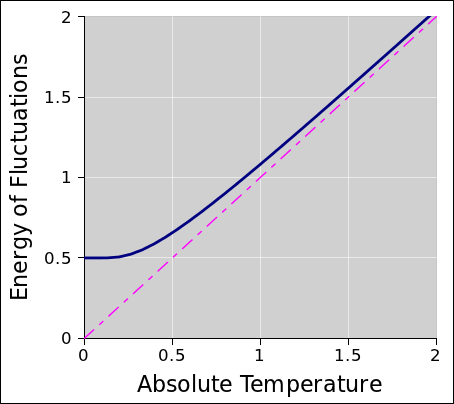
Using methods described in section 24.2 we can easily the energy of the harmonic oscillator in thermal equilibrium. The result is given by equation 24.16 and diagrammed in figure 24.1.
| (24.16) |
The entropy of a harmonic oscillator is:
| (24.17) |
In the high temperature limit (β → 0) this reduces to:
| (24.18) |
The microstates of a harmonic oscillator are definitely not equally populated, but we remark that the entropy in equation 24.18 is the same as what we would get for a system with e kT/ℏω equally-populated microstates. In particular it does not correspond to a picture where every microstate with energy Ê < kT is occupied and others are not; the probability is spread out over approximately e times that many states.
In the low-temperature limit, when kT is small, the entropy is very very small:
| (24.19) |
This is most easily understood by reference to the definition of entropy, as expressed by e.g. equation 2.3. At low temperature, all of the probability is in the ground state, except for a very very small bit of probability in the first excited state.
For details on all this, see reference 54.
Suppose we have a two-state system. Specifically, consider a particle such as an electron or proton, which has two spin states, up and down, or equivalently |↑⟩ and |↓⟩. Let’s apply a magnetic field B, so that the two states have energy
| (24.20) |
where µ is called the magnetic moment. For a single particle, the partition function is simply:
| (24.21) |
Next let us consider N such particles, and assume that they are very weakly interacting, so that when we calculate the energy we can pretend they are non-interacting. Then the overall partition function is
| (24.22) |
Using equation 24.9 we find that the energy of this system is
| (24.23) |
We can calculate the entropy directly from the workhorse equation, equation 2.2, or from equation 24.10, or from equation 24.12. The latter is perhaps easiest:
| (24.24) |
You can easily verify that at high temperature (β = 0), this reduces to S/N = kln(2) i.e. one bit per spin, as it should. Meanwhile, at low temperatures (β → ∞), it reduces to S = 0.
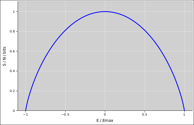
It is interesting to plot the entropy as a function of entropy, as in figure 24.2.
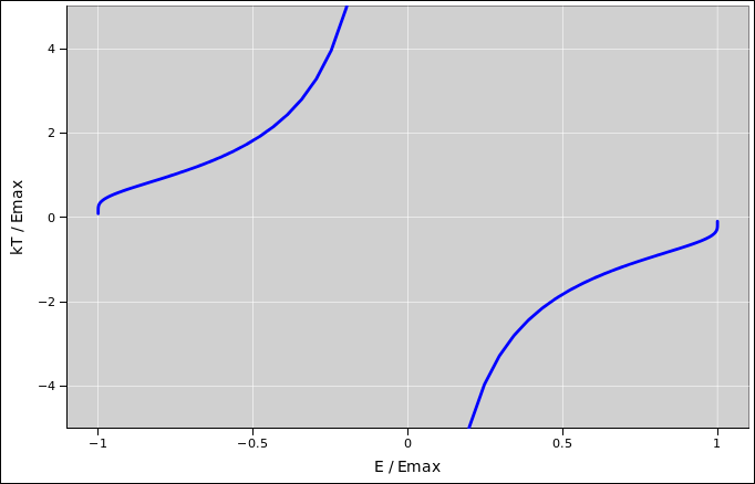
In this figure, the slope of the curve is β, i.e. the inverse temperature. It may not be obvious from the figure, but the slope of the curve is infinite at both ends. That is, at the low-energy end the temperature is positive but only slightly above zero, whereas at the high-energy end the temperature is negative but only slightly below zero. Meanwhile, the peak of the curve corresponds to infinite temperature, i.e. β=0. The temperature is shown in figure 24.3.
In this system, the curve of T as a function of E has infinite slope when E=Emin. You can prove that by considering the inverse function, E as a function of T, and expanding to first order in T. To get a fuller understanding of what is happening in the neighborhood of this point, we can define a new variable b := exp(−µB/kT) and develop a Taylor series as a function of b. That gives us
| (24.25) |
which is what we would expect from basic principles: The energy of the excited state is 2µB above the ground state, and the probability of the excited state is given by a Boltzmann factor.
Let us briefly mention the pedestrian notion of “equipartition” (i.e. 1/2 kT of energy per degree of freedom, as suggested by equation 25.7). This notion makes absolutely no sense for our spin system. We can understand this as follows: The pedestrian result calls for 1/2 kT of energy per quadratic degree of freedom in the classical limit, whereas (a) this system is not classical, and (b) it doesn’t have any quadratic degrees of freedom.
For more about the advantages and limitations of the idea of equipartiation, see chapter 25.
Indeed, one could well ask the opposite question: Given that we are defining temperature via equation 7.7, how could «equipartition» ever work at all? Partly the answer has to do with “the art of the possible”. That is, people learned to apply classical thermodynamics to problems where it worked, and learned to stay away from systems where it didn’t work. If you hunt around, you can find systems that are both harmonic and non-quantized, such as the classical ideal gas, the phonon gas in a solid (well below the melting point), and the rigid rotor (in the high temperature limit). Such systems will have 1/2 kT of energy in each quadratic degree of freedom. On the other hand, if you get the solid too hot, it becomes anharmonic, and if you get the rotor too cold, it becomes quantized. Furthermore, the two-state system is always anharmonic and always quantized. Bottom line: Sometimes equipartition works, and sometimes it doesn’t.
This section is a bit of a digression. Feel free to skip it if you’re in a hurry.
We started out by saying that the probability Pi is “proportional” to the Boltzmann factor exp(−βÊi).
If Pi is proportional to one thing, it is proportional to lots of other things. So the question arises, what reason do we have to prefer exp(−βÊi) over other expressions, such as the pseudo-Boltzmann factor α exp(−βÊi).
We assume the fudge factor α is the same for every microstate, i.e. for every term in the partition function. That means that the probability Pi† we calculate based on the pseudo-Boltzmann factor is the same as what we would calculate based on the regular Boltzmann factor:
| (24.26) |
All the microstate probabilities are the same, so anything – such as entropy – that depends directly on microstate probabilities will be the same, whether or not we rescale the Boltzmann factors.
Our next steps depend on whether α depends on β or not. If α is a constant, independent of β, then rescaling the Boltzmann factors by a factor of α has no effect on the entropy, energy, or anything else. You should verify that any factor of α would drop out of equation 24.9 on the first line.
We now consider the case where α depends on β. (We are still assuming that α is the same for every microstate, i.e. independent of i, but it can depend on β.)
If we were only using Z as a normalization denominator, having a fudge factor that depends on β would not matter. We could just pull the factor out front in the numerator and denominator of equation 24.26 whereupon it would drop out.
In contrast, if we are interested in derivatives, the derivatives of Z′ := β Z are different from the derivatives of plain Z. You can easily verify this by plugging Z′ into equation 24.9. The β-dependence matters in equation 24.9 even though it doesn’t matter in equation 24.10. We summarize this by saying that Z is not just a normalization factor.
A particularly interesting type of fudge factor is exp(−βφ) for some constant φ. You can easily verify that this corresponds to shifting all the energies in the problem by φ. This can be considered a type of gauge invariance. In situations where relativity is not involved, such as the present situation, you can shift all the energies in the problem by some constant without changing the observable physics. The numerical value of the energy is changed, but this has no observable consequences. In particular, shifting the energy does not shift the entropy.