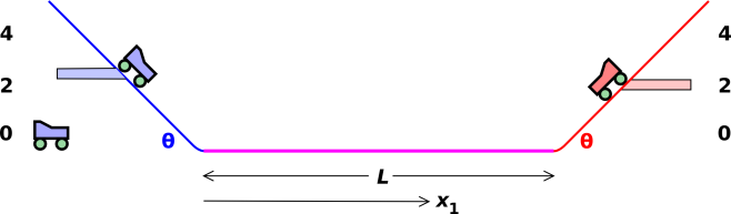
Figure 1: Carts Converging Head-On
We use the convergence of two carts as an exercise in analysis of uncertainty. We do the basic physics in section 2, and then consider the uncertainty in section 4.
Consider the situation shown in figure 1. The two carts start from rest, and then are released at the same time. Each cart rolls down a ramp to gather speed. The ramps feed into a track of length L. The carts enter at opposite ends of the track and meet somewhere in the middle. Our goal is to predict the location where they meet. (If they are in parallel lanes, they meet and pass. If they are in the same lane, they meet and collide.)
We neglect friction. This implies that the cars must be reasonably streamlined, and that the track must not be unduly long.
Let h1 represent the vertical distance that the center-of-mass of cart #1 descends as the cart moves down the ramp. This descent results in a velocity
| (1) |
and requires a time
| (2) |
where θ is the angle of the ramp, measured from horizontal. Corresponding expressions apply to cart #2.
The convergence will occur at a time
| (3) |
where x1 is the distance traveled by cart #1 on the horizontal track, after leaving the ramp. Solving for x1 we find
| (4) |
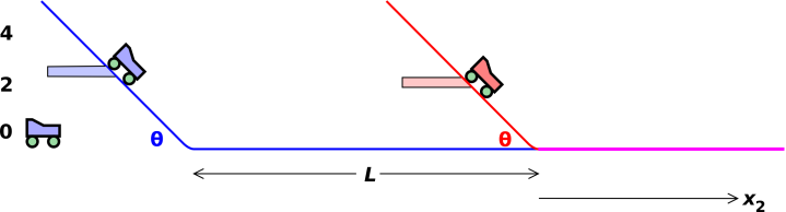
This section we consider the situation where both carts are moving in the same direction, and one overtakes the other. The slower cart is given a head start of length L. See figure 2.
The analysis is virtually identical to what we saw in section 2.1. Here we focus attention on x2, which is the distance covered by cart #2 (unlike section 2.1, which focused on x1). The convergence-point is:
| (5) |
For simplicity, we are neglecting the length of the carts. This is appropriate if the carts are in parallel lanes. (You can easily add a correction term to handle the case of a nose-to-tail collision if you want.)
Before addressing the issue of uncertainty, let’s summarize what we have already done. We have constructed a model that depends on four parameters, namely {h1, h2, θ, and L}. For any given set of parameter values, the behavior of the model is completely deterministic.
This is of course a simplified, idealized model, not nearly as complex as the real world.
Now let’s begin to think about uncertainy. As always, there are three possibilities, broadly speaking:
| Level 0: It may be that there is no significant uncertainty. It is entirely possible that the model is sufficiently faithful to the real physics, and the parameters are sufficiently precisely known, that whatever uncertainty remains is so small that nobody cares. | You should always be alert for this possibility! It would be a waste of time and resources to do an elaborate uncertainty analysis if nobody cares about the answer. We call this the deterministic level. |
| Level 1: It may be that the dominant contribution to the overall uncertainty comes from imprecise measurements of the parameters – in our example, {h1, h2, θ, and L}. | At this level – the parametric level – there are cut-and-dried methods for analyzing the uncertainty. In our example, it is possible to predict the distribution of convergence-points. |
| Level 2: It may be that the dominant contribution to the overall uncertainty come from physics that is not covered by the model. In our example, there is surely some amount of friction in the wheel bearings. There is surely some air friction, and this is particularly hard to account for, because it is sensitive to air currents. | This level – the nonparametric level – is much more open-ended. The usual procedure is to cobble up a more faithful model, which moves the problem back to level 1. However, model-building is a tremendous challenge. It requires time and effort. It requires judgment and skill. |
In introductory courses, level 1 is often heavily emphasized, at the expense of level 0 and level 2. This is partly understandable, because the parametric methods are worth learning ... but it is also a bit of a swindle, because it overestimates the power, scope, and reliability of parametric methods. Also, it simultaneously overestimates the effort required for a level-0 real-world analysis, and underestimates the effort required for a level-2 real-world analysis.
We are now going to follow the overly-well trodden path and create a situation where the parametric uncertainty is dominant.
In order to give a simplified demonstration of parametric methods for uncertainty analysis, we introduce some artificial uncertainty in the parameters. This will ensure that the dominant contribution to the uncertainty in the outcome is something we can easily identify and understand.
Building upon the deterministic model discussed in section 2, we create an ensemble of such models. Each element of the ensemble will have different values for h1 and h2. It must be emphasized that any particular element of the ensemble is completely deterministic; the uncertainty is in the ensemble, not in any particular element drawn from the ensemble.
Specifically, we arrange for h1 to be uniformly distributed over the interval from 2.25 to 2.75 units of height. This is shown by the light-blue shaded range of heights in figure 1. At the same time, we arrange for h2 to be uniformly distributed over the interval from 1.75 to 2.25 units of height. This is shown by the light-red shaded range of heights in figure 1. We can write these intervals as 2.5±0.25 and 2±0.25 if we keep in mind that the distributions are flat, not Gaussian.
Suppose we do the experiment N times, for some large value of N. We set up the carts with randomly-selected heights, let them run, and measure the convergence point. We analyze the results in various ways, including scatter plots, histograms, and cumulative probability plots. In this context, probability just means frequency; we assign 1/Nth of a unit of probability to each observed result.
We can do the experiment with real carts, or we can simulate it by using a computer to evaluate the model. We expect the distribution of computed results to closely resemble the distribution of real results, because the scatter in the initial conditions (h1 and h2) dominates other sources of uncertainty. Among other things, we can use the computed results to predict the real-world results.
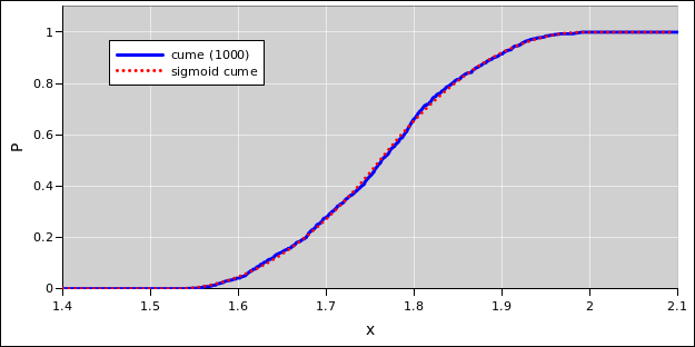
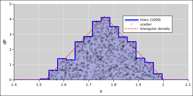
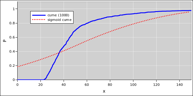
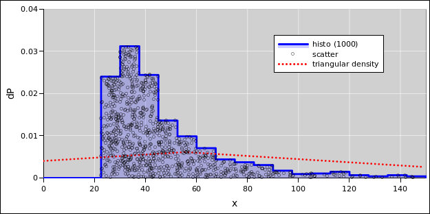
In any case, for N=1000 the results should look something like the computed results in figure 3 and figure 4. The distribution be described as approximately triangular, as you can see by comparing to the red dotted line in the figure. This triangle represents a probability density with the same mean and standard deviation as the 1000-point sample.
|
| |
| Figure 3: Distance to Head-On Convergence | Figure 4: Distance to Head-On Convergence | |
| Cumulative Probability Distribution | Probability Density Distribution |
By way of analogy: If you roll one die, the distribution of outcomes is rectangular. If you roll two dice and add the numbers, the distribution of outcomes is triangular. So, to the extent that the convergence time depends on the sum of two speeds, it is not entirely implausible that we see an approximately triangular distribution.
However, things are not really so simple. The energy of each cart follows a rectangular distribution, but the speed does not. Speed is a nonlinear function of energy. On top of that, the convergence location is a nonlinear function of the two speeds. It is something of a fluke that the worst of the nonlinearities cancel out. This will become obvious in section 4.2.
Also note that a Gaussian distribution is rather similar to a triangle. That means the distribution of convergence points could kinda maybe sorta be described as a Gaussian. However, there is no advantage to doing so. Compared to the triangular approximation, the Gaussian is in some ways worse and in no ways better.
If you are dealing with convergence physics in the real world, you cannot assume that every convergence will be head-on. The overtaking scenario is at least as important, and cannot be neglected. The basic physics is essentially identical, as you can see by comparing equation 4 and equation 5. It’s just a “distance = rate × time” problem.
Using the same methods as in section 4.1, we can find the distribution of convergence locations in the overtaking scenario. The results are shown in figure 5 and figure 6.
|
| |
| Figure 5: Distance to Rear-End Convergence | Figure 6: Distance to Rear-End Convergence | |
| Cumulative Probability Distribution | Probability Density Distribution |
This distribution cannot be approximated by a Gaussian. It cannot be approximated by a symmetric triangle. It cannot be approximated by any kind of triangle. The distribution has a mean and a standard deviation, but those don’t tell you very much about the shape and significance of the distribution. The dotted red line in figure 5 and figure 6 represents a triangular probability density with the same mean and same standard deviation as the 1000 computed points. It is dramatically dissimilar to the actual distribution, partly because the mean and standard deviation are strongly affected by the presence of a few exceedingly long convergence times.
The messy distribution in section 4.2 must not be blamed on the artificial spread in the parameters h1 and h2. In fact, if there were no artificial spread, the distribution of convergence-points would still be messy, and the mess would be harder to understand.
The root of the problem is the fact that the deterministic mechanics is a nonlinear function of the parameters h1 and h2, as we can see in equation 5.
Any analysis method that can handle cart #2 westbound but not eastbound is not a reliable method.
The spreadsheet used to create the probability diagrams is given in reference 1.
For details on how to represent uncertainty, see reference 2. For some explanation of the techniques used to create the probability diagrams, see reference 3. For the basic concepts and terminology of probability, see reference 4.