Figure 1: Flux Tubes
You presumably know how to visualize a magnetic field in terms of “magnetic lines of force” aka “magnetic flux lines”. As we shall see, this is a powerful but imperfect idea. We will briefly review the idea, then discuss its limitations, and then explain how to replace it with a similar but much better idea, namely flux tubes.
Suppose our observer, Joe, goes into the laboratory and observes that in a particular region of space, there is a magnetic field in the Z direction. That is, the magnetic field B has a nonzero Bz component, while the Bx and By components are zero. We can visualize this as a set of magnetic field lines, equally spaced, all running in the Z direction.
In this scenario, there is no E field, according to Joe.
Flux lines are like contour lines on a topographic map, in the following sense: When a slope is more intense, the contour lines are closer together. When a magnetic field is more intense, the magnetic field lines are closer together.
We can quantify this in terms of flux, as follows: Given a patch of surface, we can calculate the magnetic flux through that surface, namely the number of field lines that penetrate the given surface. Since our field is in the Z direction, there will be a nonzero flux through a surface oriented parallel to the XY plane, but no flux through any surfaces oriented parallel to the YZ or ZX planes.
As we shall see, the thing that the old approach called a magnetic field vector in the Z direction should really be called a magnetic (or electromagnetic) field 2-form in the n XY direction. The fact that the old-style field lines seem to “flow” in the Z direction is much less important than the fact that they penetrate the XY surfaces. A charge moving in the XY plane is affected by an XY magnetic field, while a charge moving in the Z direction is not. The symmetry of the field is an XY symmetry, not a Z symmetry, as discussed in reference 1.
To say the same thing another way, if the old approach called it a pure magnetic field vector in the Z direction, the new approach calls it an electromagnetic field 2-form that is active purely in the XY plane.
That is all fine as far as it goes.
Alas, a slight problem arises if we ask how things look to a different observer, Moe, who is using a reference frame that is moving relative to Joe’s reference frame. In the region of interest, Moe will observe a different amount of magnetic field, and will also observe a nonzero electric field.
We conclude from this that magnetic field lines do not have direct physical significance, because different observers disagree on how many of them there are. Specifically, even if you can draw magnetic field lines in ordinary three-dimensional space, you cannot draw magnetic field lines in spacetime.
We have seen this situation before, in connection with vectors. Suppose we have a vector relationship such as P = Q + R. If we have two observers, using reference frames that are rotated relative to one another, they will disagree about the numerical value of the components of these vectors. On the other hand, all observers agree that P is the sum of Q and R. We can add Q and R graphically, tip to tail, without reference to any coordinate systems. This is explained in much greater detail in reference 2.
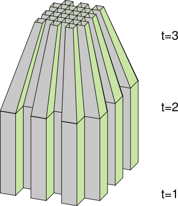
We can greatly improve the situation by considering electromagnetic flux tubes instead of flux lines. We shall see that the electromagnetic flux tubes have direct physical significance. An example is shown in figure 1.
In this diagram, we show only the timelike direction and two spacelike directions; the third spacelike direction is suppressed.
On the left side of the diagram, we see a bundle of tubes. We emphasize that these tubes have physical significance in spacetime, independent of any coordinate system.
However, having said that, we can also say a few words about how those flux tubes are oriented relative to the laboratory frame, as shown on the right side of the figure. In fact, we find that this bundle of tubes is precisely transverse to the XY plane. The tubes seem to be “flowing” in the T direction. Indeed they are “flowing” in the T and Z directions, but you cannot easily see that, because the Z direction has been suppressed in this diagram.
In any case, as foreshadowed above, the direction of “flow” is not nearly as important as the direction of activity. The field pictured in figure 1 is active in the XY plane. The XY component of field strength is measured by counting how many flux tubes there are per unit area in the XY plane.
It turns out that whenever the electromagnetic field F is active in a spacelike plane (in a particular frame), we call it a magnetic field (in that frame). This means that the tubes shown in figure 1 can be identified – in the lab frame – as a purely magnetic field, with the old-style B vector aligned in the Z direction. Using the new style, we say it is active in the XY plane.
In contrast, an electromagnetic field that is active in a timelike plane is called an electric field (in the given frame). Specifically:
All observers agree on what the flux tubes are doing, even if they don’t agree on which part to call “electric” and which part to call “magnetic”.
Let’s be clear: In spacetime there is no electric field (E) per se and no magnetic field (B) per se; there is only the electromagnetic field (F). In any particular reference frame, you can identify an electrical part and a magnetic part within the electromagnetic field, but this identification is frame-dependent.
In spacetime, electrical flux tubes are the same as magnetic flux tubes, except for orientation.
You presumably know that old-style magnetic field lines are endless. You can twist them and stretch them like rubber bands, but you cannot break them.
In spacetime, the corresponding statement is that in the absence of electrical charge, the electromagnetic tensor F is represented by flux tubes that are endless in space and time.
In figure 1, you can see what might be called “ends” of the tubes, but that is entirely artificial. That is because, for clarity, we are showing only a section of the tubes, namely the section starting at t=1 and ending at t=2. If we showed the full time history, the tubes would be endless.
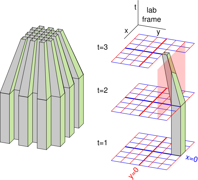
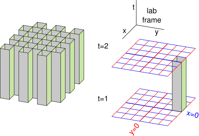
Figure 3 shows an example of an electromagnetic field that is not constant.
In the lab frame, the situation can be described as follows: Initially, the magnetic field is constant (between time t=1 and time t=2) and then it changes (between time t=2 and time t=3).
The final magnetic field is fourfold stronger than the initial field. That is, there are four times as many flux tubes per unit area in the XY plane.
The Maxwell equations tell us that (in any particular frame) the electric field is not independent of the magnetic field. In particular, if there is a time-varying magnetic field, there must also be an electric field.
This constraint can be understood as a direct consequence of the endlessness discussed in section 1.3. An example is shown in figure 3.
On the right side of the diagram, we follow just one of the tubes. One of its corners starts at x=0, y=0.4 and ends up at x=0, y=0.2. The interesting thing is that in the process, the tube must cross a plane that is parallel to the TX direction, such as the plane shown in pale transparent red in the diagram. That is to say, the tube is active in the TX direction. Therefore, at certain locations, such as the x=0, y=0.4 location, there is a nonzero electric field. If we represent this by an old-style E vector, it points the X direction.
Overall, the direction of the induced electric field is azimuthal. That is, when x is large, the old-style E vector is in the +Y direction, and when y is large, the old-style E vector is in the −X direction.
In the situation we are considering, at the center of symmetry (x=0, y=0) there is no electric field, even when the magnetic field is changing.
To summarize: The four-dimensional geometry of endless tubes guarantees that you cannot have an electromagnetic field that is changing and purely magnetic. If it is magnetic and it is changing, it is also electric, except perhaps at one special point.
We have explained why this must be true in the absence of electrical charge. It is also true even when there is some charge, but the explanation is more complicated.
Consider the common situation where we have a long solenoid. Far from the ends of the solenoid, the B field is spatially uniform inside the solenoid and essentially zero in the neighboring regions. We increase the flux inside the solenoid by increasing the current. The structure and shape of the solenoid stay the same.
Beware that figure 3 is not a good a good model of this situation. There is no region in the figure where the B field is uniformly increasing inside the region and zero outside the region.
The figure represents something like the following situation, which might occur in a magnetohydrodynamics experiment: suppose we have some flux lines trapped in a plasma, and we compress the plasma.
Alternatively, you can try to “fix up” figure 3 in your mind’s eye, to make it more representative of an ordinary solenoid. As the bundle of tubes shrinks, imagine bringing in additional tubes from far, far way. Bring in enough tubes to maintain the size of the bundle. The added tubes were initially very large tubes (corresponding to very small magnetic field intensity) and were initially very far away, so they are consistent with the requirement that the magnetic field be nearly zero outside the solenoid.
These added tubes, rushing in from far, far away, are highly active across TR surfaces in the vicinity of the solenoid, where R is the radial coordinate. That is to say, there will necessarily be a significant induced E field both inside the solenoid and in the nearby regions.
I have left out several details. For starters, the diagrams do not distinguish +F from −F. This would be not be hard to fix, but I haven’t got around to it yet.
If you want the next level of detail, an excellent reference for the spacetime view of electromagnetism – both the pictures and the math – is chapter 4 of reference 3.
Beware that the F used here and in reference 3 is different from the F used in reference 4 and elsewhere. Here it is a two-form; elsewhere it is a bivector. This affects the pictures but not the mathematics, since there is a one-to-one mapping between the two representations.