Figure 1: Lorentz Law
Electromagnetism using Geometric Algebra versus Components |
The task for today is to compare some more-sophisticated and less-sophisticated ways of expressing the laws of electromagnetism. In particular we compare Geometric Algebra, ordinary vectors, and vector components.
We do this in the spirit of the correspondence principle: whenever you learn a new formalism, you should check that it is consistent with what you already know.
This document is also available in PDF format. You may find this advantageous if your browser has trouble displaying standard HTML math symbols.
As we shall see in section 5, Maxwell’s equations for the electromagnetic field can be written in the remarkably compact and elegant form:
| ∇ F = |
| J (1) |
where J a vector in spacetime, representing the charge and current, and F is a bivector, representing the electromagnetic field. It is worth learning the geometric algebra (aka Clifford algebra) formalism just to see this result.
It is also interesting to apply the correspondence principle, to see how this equation reproduces results that may be more familiar in other forms. Therefore let’s take a step back and review the prosaic non-spacetime non-geometric version of Maxwell’s equation.
We start by writing the Maxwell equations in terms of vector fields in three dimensions, namely:
| (2) |
These equations have several deep symmetries. We can make some of the symmetries more apparent by making a few superficial changes. The reasons for this will be explained in moment.
| (3) |
These equations are invariant with respect to rotations in three dimensions. They are manifestly invariant, because they have been written in vector notation. We have not yet specified a basis for three-dimensional space, so if Alice uses a reference frame that is that is rotated relative to Bob’s reference frame, equation 3 not only means the same thing to both of them, it looks the same, verbatim.
These equations have an additional invariance, an invariance that is important but not manifest, namely relativistic invariance. The invariance is hidden because, among other things, the t coordinate appears explicitly. If Alice uses a reference frame that is moving relative to Bob’s reference frame, they won’t be able to agree on the value of t. For that matter, they won’t be able to agree on the values of the E-field and B-field.
Of course the non-agreement about the coordinates and the non-agreement about the fields cancel in the end, so Alice and Bob eventually agree about what the equations predict will happen physically.
Therefore equation 3 represents an intermediate level of sophistication: manifest invariance with respect to rotations, but non-manifest invariance with respect to boosts.
In passing from equation 2 to equation 3, we added factors of c in strategic places. This helps make the equations more manifestly symmetric. Specifically:
Some tangential remarks:
We can construct an even-less-sophisticated expression by choosing a basis and writing out the components:
| (4) |
See section 10.1 for information about the notation used here.
Expressing things in components like this is sometimes convenient for calculations, but it conceals rotation-invariance. If Alice uses a reference frame that is rotated relative to Bob’s, they won’t be able to agree on what xi means or what Ei means. Of course the rotation-invariance is still there; it has just become non-manifest.
Geometric Algebra (also known as Clifford Algebra) has many advantages, as discussed in section 8. It turns out we can write the Maxwell equations in the easy-to-remember form
| ∇ F = |
| J (5) |
which contains the entire meaning of the less-sophisticated version, equation 3, as we shall demonstrate in a moment.
This expression has the advantage of being manifestly Lorentz invariant (including boosts as well as rotations). Contrast this with equation 3 in which the Lorentz invariance is not manifest.
Overall, the best approach would be to solve practical problems by direct appeal to equation 1. Some examples can be found in section 11 and reference 3.
However, that’s not the main purpose of this document. Instead, we want to derive the less-sophisticated Maxwell equations (equation 3) starting from equation 1. This can be considered a test or an application of the correspondence principle.
For starters, we need to establish the correspondence between the 3-dimensional electric current j and the corresponding four-vector current J. That is,
| J = c ρ γ0 + jk γk (6) |
where we have chosen a reference frame in which γ0, γ1, γ2, and γ3 are the orthonormal basis vectors. In particular, γ0 is the timelike basis vector. We see that ρ has to do with continuity of flow of charge in the time direction, just as the ordinary three-dimensional current j represents flow in the spacelike directions. See reference 4 for more about the idea of conservation and continuity of flow.
We also need to know how F is related to the old-fashioned fields E and B. In any particular frame,
| (7) |
where i is the unit pseudoscalar (equation 48). We can expand this as:
| (8) |
where Ek and Bk are the components of the old-fashioned electric field and magnetic field as measured in our chosen frame.
If we write the basis vectors in dictionary order, we have:
where only the y-component of B gets a + sign. It is sometimes convenient to swap the basis vectors on this one term, whereupon we can write:
so that everybody gets a − sign. Mnemonic: This makes the superscripts and subscripts in each term of equation 10a become cyclic permutations of (123). The notion of cyclic order makes sense in some situations but not others; for starters, it does not apply to equation 10a.
Tangential remark: We can also write equation 8 in terms of the Hodge dual, as explained in section 10.3.
F = E γ0 − cB §E (11)
The equations in this section have quite an interesting structure. They tell us we ought to view the electromagnetic field as a bivector. In any particular frame this bivector F has two contributions: one contribution is a bivector having one edge in the timelike direction, associated with E, while the other contribution is a bivector having both edges in spacelike directions, associated with cB.
We are making heavy use of the central feature of the Clifford Algebra, namely the ability to multiply vectors. This multiplication obeys the usual associative and distributive laws, but is not in general commutative.1 In particular because our basis vectors γµ are orthogonal, each of them anticommutes with the others:
| γµ γν = − γν γµ for all µ ≠ ν (12) |
and the normalization condition2 in D=1+3 requires a minus sign in the timelike component:
| γ0 γ0 = −1, γ1 γ1 = +1, γ2 γ2 = +1, γ3 γ3 = +1 (13) |
Now all we have to do is plug equation 7 into equation 1 and turn the crank.
There will be 12 terms involving E, because E has three components Ek and the derivative operator has four components ∇µ. Similarly there will be 12 terms involving B.
| (14) |
Let’s discuss what this means. We start with the nine terms highlighted in blue. The six terms involving cB are the components of ∇ × cB. Similarly, the three terms involving E are the components of +∇0 E, which is the same as −(∂/c∂t) E. These terms each involve exactly one of the spacelike basis vectors (γ1, γ2, and γ3), so we are dealing with a plain old vector in D=3 space. The RHS of the equation 1 has a vector that matches this, namely the D=3 current density. So the blue terms are telling us that ∇ × cB − (∂/c∂t) E = (1/cє0) j, which agrees nicely with equation 3.
Next, we consider the nine terms highlighted in red. The six terms involving E are the components of ∇ × E. Similarly, the three terms involving cB are the components of −∇0 cB, which is the same as +(∂/c∂t) cB. These nine terms are all the trivectors with a projection in the timelike direction (γ0). Since the RHS of equation 1 doesn’t have any trivector terms, we must conclude that these red terms add up to zero, that is, ∇ × E + (∂/c∂t) cB = 0, which also agrees with equation 3.
The three black terms involving E match up with the timelike piece of J and tell us that ∇ · E = (1/є0) ρ. The three black terms involving cB tell us that ∇ · cB = 0.3
Let me say few words about how this was calculated. It really was quite mechanical, just following the formalism. Consider the term +∇2 cB3 γ1 in the last row. We started from the expression ∇ F which has two factors, so the term in question will have two factors, ∇2γ2 and −cB3γ3 γ1γ2γ3, which combine to make −∇2γ2cB3γ3γ1γ2γ3. All we have to do is permute the γ vectors to get this into standard form. Pull the scalars to the front and permute the first two vectors using equation 12 to get +∇2cB3γ3γ2γ1γ2γ3. Permute again to get −∇2cB3γ3γ1γ2γ2γ3 which reduces using equation 13 to −∇2cB3γ3γ1γ3. Then one more permutation and one more reduction and the job is done.
The only part that required making a decision was writing γ0γ3γ1 in places where I could have written −γ0γ1γ3. This is just cosmetic; it makes the signs fall into a nice pattern so it is easier to see the correspondence with the old-fashioned cross product. We can make this seem more elegant and less arbitrary if we say the rule is to write all pseudovectors using the basis {i γµ for µ=0,1,2,3}, where i is the unit pseudoscalar (equation 48).
After the calculation was done, deciding how to color the terms took some judgment, but not much, because the terms naturally segregate as vectors and trivectors, spacelike and timelike.
Preview: Our goal is to prove that charge is conserved, i.e. that ∇·J=0. We are not going to assume conservation; we are going to prove that conservation is already guaranteed as a consequence of equation 1, the Maxwell equation. We will do that by taking the divergence of both sides of the equation.
Background: We are going to need a mathematical lemma that says the divergence of the divergence of a bivector is always zero. To derive this, consider an arbitrary bivector W. We temporarily assume W is a simple blade, i.e. W = a γ5 γ6. Then the divergence is
| (15) |
where on the second line we have used the general rule that the dot product is the low-grade piece of the full geometric product. On the last line we have temporarily assumed that γ5 and γ6 are spacelike, but we shall see that this assumption is unnecessary.
Let us now take the divergence of the divergence.
| (16) |
On the last line we have used the fact that the various components of the gradient operator commute with each other.
We now lift the assumption that our basis vectors are timelike. You should verify that it doesn’t really matter whether γ5 and γ6 are spacelike or timelike. Hint: a fuller calculation would give us:
| (17) |
We now lift the assumption that W is a blade. By the distributive law, if ∇·(∇·W) is zero for any grade=2 blade, it is zero for any sum of such blades, i.e. for any bivector whatsoever. We conclude in all generality:
| (18) |
As another lemma, for any bivector we can always write
| (19) |
This allows us to pick apart ∇F as follows:
|
For the purposes of this section, all we need is equation 20b. That is the grade=1 piece of the Maxwell equation. We do not need to assume the non-existence of monopoles. We do not need to know anything about the trivector piece of the Maxwell equation. We do not need equation 20d or even equation 20c.
Using our lemma (equation 18), we can write
| (21) |
We are of course using the four-dimensional divergence. Zero divergence expresses the continuity of world-lines in spacetime. For an explanation of why this is the right way to express the idea of conservation in terms of continuity of flow, see reference 4.
As remarked above, our theory of electromagnetism would be incomplete without the Lorentz force law.
The old-fashioned way of writing the Lorentz force law is:
| p = q(E + |
| × cB) (22) |
where p is the momentum, q is the charge, and v is the ordinary 3-dimensional velocity.
As with practically any equation involving cross products, equation 22 can be improved by rewriting it using Geometric Algebra instead:
| p = q u · F (23) |
where τ is the proper time, u = dx/dτ is the 4-dimensional proper velocity,4 p = m u is the momentum, and m is the invariant mass. Here p and u are vectors in D=1+3 spacetime. This is the relativistically-correct generalization of equation 22.
Equation 23, unlike previous equations, involves a dot product. In particular, it involves the dot product of a vector with a bivector. Such things are not quite as easy to compute as the dot product between two vectors, but they are still reasonably easy to compute in terms of the geometric product. In general, the dot product is the lowest-grade part of the full geometric product, as discussed in reference 5. In the case of a vector dotted with a bivector, we have:
| (24) |
That means we just form the geometric product and throw away everything but the grade=1 part. Another way of dealing with “vector dot bivector” is:
| (25) |
which can be considered a sort of “distributive law” for distributing the dot-operator over the wedge-operator. Equation 25 tells us that the product A·(B∧C) is a vector that lies in the plane spanned by B and C.
The following examples are useful for checking the validity of the foregoing equations:
| (26) |
To say the same thing in geometric (rather than algebraic) terms, you can visualize the product of a vector with a bivector as follows:
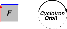
An example of the Lorentz law in action is shown in figure 1, for the case of an electromagnetic field bivector (F) that is uniform in space, oriented purely in the plane of the paper. The cyclotron orbit shown in the figure corresponds to the motion of a positive test charge with some initial velocity, free of forces other than the indicated electromagnetic field.
It is straightforward to understand this result. If the particle is moving in the direction of the red vector, it will experience a force in the blue direction. If the particle is moving in the blue direction, it will experience a force opposite to the red direction.
To summarize: The magnetic part of the Lorentz force law is super-easy to remember:
| |
Motion perpendicular to the field bivector is unaffected by the field.
The foregoing applies if the field F is already expressed in modern terms, as a bivector. Now, in the spirit of this document, we re-examine the situation to exhibit the correspondence between the bivector idea and old-fashioned ideas such as the electric field vector and the magnetic field pseudovector.
The bivector shown in figure 1 is purely spatial, so it must correspond to a magnetic field, with no electric field in our frame of reference. The magnetic field pseudovector is perpendicular to the paper, directed out of the paper. You can check using the right-hand force rule that the cyclotron orbit shown in figure 1 is correct for a positive test charge moving in such a magnetic field.
It is amusing to check the general case, for any F that is known in terms of the old-fashioned electric field vector and magnetic field pseudovector, as in equation 7 or equation 8. As suggested by equation 23, we should take the dot product of u with both sides of our expression for F. The correspondence principle suggests we should recover the old-fashioned 3-vector version of the force law, i.e. equation 22. To carry out the dot product, we could just turn the crank ... but in fact we hardly need to do any work at all. The dot product in u · F uses a subset of the full geometric product u F, namely the plain vector (grade=1) terms. See equation 18 in reference 6. We can avoid some work, because u F has the same structure as ∇ F – it’s just the geometric product of some vector with F – so we can just re-use equation 14, replacing ∇ by u everywhere. Then we throw away all the trivector terms, and what remains is the dot product.
In the nonrelativistic limit, the timelike component of the velocity equals unity, plus negligible higher-order terms. So the blue terms in equation 14 give us the usual Lorentz equation for the spacelike components of the momentum-change: 1 E + v × B.
The black terms involving E give us a bonus: They tell us the power (i.e. the rate of work, i.e. the time-derivative of the kinetic energy), namely v · E.
Let us consider the gorm of the electromagnetic field, namely gorm(F) ≡ ⟨FF ∼⟩0. You can readily verify that:
| ⟨FF ∼⟩0 = (cB)2 − E2 (27) |
This is a scalar, a Lorentz-invariant scalar. It is useful in a number of ways, not least of which is the fact that −є0((cB)2 − E2) is the Lagrangian density for the electromagnetic field.
Let’s continue looking for energy-related expressions involving F. Section 6.3 gives us hint as to where to look; the Lagrangian density is not “the” energy density, but it at least has dimensions of energy density.
We know from old-fashioned electromagnetism that there should be an energy density that goes like the square of the field strength. This tells us the amount of energy per unit volume. In old-fashioned terms, the energy density is ½ є0 (E2 + c2 B2).
There is also a Poynting vector, which tells us the amount of energy flowing per unit surface area, per unit time. In old-fashioned terms, it is c є0 E×cB. .
So, without further motivation, we use 20/20 hindsight to assert that F γ0 F will be interesting. Following the spirit of this document, let’s check that assertion by working out F γ0 F in terms of the old-fashioned E and B fields, and seeing what we get. We substitute for F using equation 7 and turn the crank:
| (28) |
In going from the second line to the third line, we used the fact that (γ0)2 = −1. We also used the fact that γ0γk = − γ0γk for all k ∈ {1,2,3}. On the other hand, (γ1γ2γ3)γk = +γk(γ1γ2γ3). That is, when we commute γk across the three factors in (γ1γ2γ3), we pick up only two factors of −1, not three, since for one of the factors the subscript on that factor will match the subscript k, and γk obviously commutes with itself.
In the next step, we used the fact that (γ1γ2γ3)2 = −1. We also changed some dummy indices.
So we see that we should be particularly interested in the quantity
| (29) |
The spacelike part of T(γ0) is the old-fashioned three-dimensional Poynting vector (apart from a missing factor of c), while the timelike component represents the corresponding energy density.
Although this T(γ0)-vector has four components, it is not a well-behaved Lorentz-covariant four-vector. It is actually just one column of a 4×4 object, namely the stress-energy tensor, T. Writing T(γ0) in terms of E and B (as in the second line of equation 29) only makes sense in the particular frame where E and B are defined. Also, if you want to connect T(γ0) to the Poynting vector in a given frame, γ0 cannot be just any basis vector, but must be the 4-velocity of the frame itself, i.e. the unit vector in the time direction in the given frame.
More generally, the quantity
| T(a) := −½ є0 F a F (30) |
represents the flow of [energy, momentum] across the hypersurface perpendicular to the vector a. A more general way of looking at this is presented in section 6.5.
The stress-energy tensor T for the electromagnetic field (in a vacuum) has the following matrix elements:
| Tµν = F γµF γν (31) |
for any set of basis vectors {γµ}. Equation 29 and equation 30 can be understood as special cases of equation 31.
In four dimensions, the electromagnetic field bivector F can always be written as the exterior derivative of a quasi-vector-ish potential A. Conversely, we can integrate the electromagnetic field to find the potential difference between point P and point Q.
| (32) |
This implicitly defines what we mean by A. However, A is not uniquely defined, as discussed in section 7.3. Furthermore, even though A looks like it might be a four-vector, it’s not.
Conversely, you can always integrate the electrostatic field to find the potential difference between any two points.
| (33) |
That suffices to prove that:
| (34) |
This tells us that any attempt to integrate E to find the scalar potential difference between point P and point Q will fail; the integral will depend on the path from P to Q, not just on the endpoints.
| (35) |
|
However, beware that equation 36a is a swindle, because it defines an object that is not a four-vector. It has four components, but that is not sufficient to make it a well-behaved 4-vector. It does not behave properly with respect to Lorentz transformations.
This is not tragic, because the potentials are not directly observable. The only thing that matters is the difference between two potentials, and that turns out to be well behaved, for the following reason:
Loosely speaking, if you start out with a vector-ish potential in a certain gauge and then change to a different reference frame, you get a vector-ish potential with the same physical meaning in some other screwy gauge. If you try to calculate A by evaluating it in one frame and then boosting it into another frame, you will almost certainly get the wrong value for A. However, when you compute any physical observable, the gauge drops out, so you might end up with the right physics.
In particular, the key equation 32 is OK. The electromagnetic field F is a well-behaved bivector. The exterior derivative on the RHS annihilates any and all gauge fields.
In any case, if you choose a particular reference frame and a particular gauge, then you can think of ϕ/c as being the timelike component of A.
At this point you should be asking yourself, how can ∇∧(field) be nonzero in three dimensions but zero in four dimensions? How does that not violate the correspondence principle? How does that not contradict the claim made in reference 7 that Minkowski spacetime is very very similar to Euclidean space?
The answer is that when we switch from three dimensions to four, we redefine mean by “the” field, “the” potential, and “the” wedge product. In four dimensions, the exterior derivative of a vector has more terms. Invoking the correspondence principle, we can explain this in terms of the old-style E and B fields as follows: when we compute ∇∧F, the time derivative of the B-component cancels the spatial derivatives of the E-component.
This is a trap for the unwary. Don’t let your experience with D=3 poison your intuition about D=4. Consider the contrast:
| In D=3 it is important to remember that “the field” (E) is not generally the derivative of any potential. | In D=4, we can always write “the field” (F) as F = dA. |
| For some problems, there is a natural reference frame that has immense practical significance. | For some problems, the frame-independent spacetime approach is simple, convenient, powerful, and elegant. |
For example, if you are dealing with transformers or ground loops, you care a lot about the electric field in the frame of the device. The fact that this field cannot be written as the gradient of any potential is important. See reference 8 for suggestions on how to visualize what’s going on.
The vector-ish potential is implicitly defined by equation 32. However, for any given field F, you don’t know whether the vector-ish potential is A or A + λ′, since we can write:
| (37) |
for any vector field λ′ such that
| (38) |
In particular, we can use the gradient of any scalar field λ:
| (39) |
which is guaranteed to work since ∇∧∇(anything) is automatically zero. Beware of inconsistent terminology: Sometimes λ is called «the» gauge field, and sometimes λ′ is called «the» gauge field.
The fact that we can write the electromagnetic field bivector as the derivative of a vector field is related to the fact that there are no trivector terms on the RHS of the Maxwell equation (equation 1). In particular, because ∇ is a vector, we can always write:
| (40) |
Equation 40 is a mathematical identity, valid for any F you can think of. Applying it to the electromagnetic field in particular and plugging in equation 32 we obtain:
| (41) |
So we could not write F = ∇∧A unless we already knew that ∇∧F was zero, since ∇∧∇∧A is automatically zero. Indeed ∇∧∇∧(anything) is automatically zero; see equation 20.
Combining these ideas, we see that another way of writing the Maxwell equation is:
| ∇·∇∧ A = |
| J (42) |
or equivalently:
| ∇2 A = |
| J (43) |
were ∇2 is called the d’Alembertian, or (equivalently) the four-dimensional Laplacian. It’s the dot product of the derivative operator with itself.
Some references express the same idea using a different symbol:
| □2 A = |
| J (44) |
Beware that yet other references use plain unsquared □ to represent the d’Alembertian. The idea is that they reserve ∇2 to represent the three-dimensional Laplacian, and use □2 to represent the four-dimensional generalization. However, in this document, we assume that all vectors are four-dimensional unless otherwise specified; for example, p is the four-momentum, A is the four-vector-ish potential, ∇ is the four-dimensional gradient, et cetera.
Geometric Algebra has some tremendous advantages. It provides a unified view of inner products, outer products, D=2 flatland, D=3 space, D=1+3 spacetime, vectors, tensors, complex numbers, quaternions, spinors, rotations, reflections, boosts, and more. This may sound too good to be true, but it actually works.
If you need an introduction to Geometric Algebra, please see reference 9, reference 10, and other references in section 12. Just as I did not include an introductory discussion of the divergence and curl operators in equation 3, I will not include an introductory discussion of Geometric Algebra here. There’s no point in duplicating what’s in the references. In particular, reference 10 discusses electromagnetism using D=3 Clifford Algebra, which is easier to follow than the D=4 discussion here, but the results are not as simple and elegant as equation 1. The calculation here, while not particularly difficult, does not pretend to be entirely elementary.
In Geometric Algebra, it traditional to not distinguish vectors using boldface or other decorations. This is appropriate, since the Clifford Algebra operates on multivectors and treats all multivectors on pretty much the same footing. Multivectors can be scalars, vectors, bivectors, pseudovectors, pseudoscalars — or linear combinations of the above.
Observe that there is no cross-product operator in equation 1 or equation 23. That is good. Cross products are trouble. They don’t exist in two dimensions, they are worse than useless in four dimensions, and aren’t even 100% trustworthy in three dimensions. For example, consider a rotating object and its angular-momentum vector r × p. If you look at the object in a mirror, the angular-momentum vector is reversed. You can’t draw a picture of the rotating object and its angular-momentum vector and expect the picture to be invariant under reflections.
As far as I can tell, every physics formula involving a cross product can be improved by rewriting it using a wedge product instead.
For a rotating object, the cross product r × p is a vector oriented according to the axis of rotation, while the wedge product r ∧ p is an area oriented according to the plane of rotation. The concept of “axis of rotation” is not portable to D=2 or D=4, but the concept of “plane of rotation” works fine in all dimensions.
If you think cross products are trouble, wait till you see Euler angles. They are only defined with respect to a particular basis. It’s pathetic to represent rotations in a way that is not rotationally invariant. Geometric Algebra fixes this.
Note that Clifford Algebra does not require any right-hand rule. In equation 13, the timelike vector is distinguished from the spacelike vector, but otherwise that equation and equation 12 treat all the basis vectors on an equal footing; renaming or re-ordering them doesn’t matter.
In D=3 or D=1+3 the unit pseudoscalar (equation 48) is chiral; that is, constructing it requires the right-hand rule. The axioms of Clifford Algebra sometimes permit but never require the construction of such a critter. The laws of electromagnetism are completely left/right symmetric. The magnetic term in equation 7 contains B, which is chiral because it was defined via the old-fashioned cross product ... but the same term contains a factor of i which makes the overall expression left/right symmetric. It would be better to write the magnetic field as a bivector to begin with (as in reference 3), so the equations would make manifest the intrinsic left/right symmetry of the physical laws.
There are at three different approaches to defining an F-like quantity as part of a geometric-algebra formulation of electromagnetism.
Each approach is self-consistent, and most of the equations, such as equation 1, are the same across all systems.
The advantage of the bivector + bivector approach is that it is “at home in spacetime”, i.e. it treats x and t on the same footing, and treats B and E on the same footing (to the extent possible). It makes it easy and intuitive to draw bivector diagrams of the sort used in reference 3.
You may be accustomed to expanding the dot product as
| A·B ?=? A1B1 + A2B2 + A3B3 (45) |
as if that were the definition of dot product ... but that is not the definition, and you’ll get the wrong answer if you try the corresponding thing in a non-Euclidean space, such as spacetime. So what you should do instead is to expand
| A = Aµγµ = A0γ0 + A1γ1 + A2γ2 + A3γ3 (46) |
where the γµ are the basis vectors. Such an expansion is always legal. That is what defines the components Aµ. The superscripts on A label the components of A; they are not exponents. The subscripts on γ do not indicate components; they simply label which of the basis vectors we are talking about. It is possible but not particularly helpful to think of γ0 as the zeroth component of some “vector of vectors”; in any case remember that γ0 is a vector unto itself.
When you take the dot product A·B, the expansion equation 46 (and a similar expansion for B) gives you sixteen terms, since the dot product distributes over addition in the usual way. The twelve off-diagonal terms vanish, since they involve things like γ1.γ2 and the basis vectors are mutually orthogonal. So we are left with
| (47) |
where the term A0B0 has picked up a minus sign, because γ02 is -1.
Another thing to watch out for when reading the Geometric Algebra literature concerns the use of the symbol i for the unit pseudoscalar:
| i := γ0γ1γ2γ3 (48) |
It’s nice to have a symbol for the unit pseudoscalar, and choosing i has some intriguing properties stemming from the fact that i2 = −1, but there’s a pitfall: you may be tempted to treat i as a scalar, but it’s not. Scalars commute with everything, whereas this i anticommutes with vectors (and all odd-grade multivectors). This is insidious because in D=3 the unit pseudoscalar commutes with everything. For these reasons we have mostly avoided using i in the main part of this note.
Logical consistency requires that when using superscripts as exponents, they should denote simple powers:
| (49) |
for any multivector M. However, there is an unfortunate tendency for some authors to write M2 when they mean MM ∼ where M ∼ is the reverse of M, formed by writing in reverse order all the vectors that make up M; for example the reverse of equation 7 tells us that F ∼ = γ0(E+cBi).
This is insidious because for scalars and vectors MM ∼ = MM; the distinction is only important for grade-2 objects and higher.
I recommend writing out MM ∼ whenever you mean MM ∼. Many authors are tempted to come up with a shorthand for this – perhaps M2, |M|2, or ||M||2 – but in my experience such things are much more trouble than they are worth. You need to be especially careful in the case where there are timelike vectors involved, since MM ∼ might well be negative. In such a case, any notation that suggests that MM ∼ is the square of anything is just asking for trouble.
A related and very important idea is the gorm of an object M, defined to be the scalar part of MM ∼, i.e. ⟨MM ∼⟩0. (We saw a good physical example, namely the gorm of the electromagnetic field, in section 6.3.)
The dot product of a vector with a bivector is anticommutative, so be careful how you write the Lorentz force law:
| u · F = − F · u (50) |
This is insidious because the dot product is commutative when acting on two vectors, or on “almost” any combination of multivectors. It anticommutative only in cases where one of them has odd grade, and the other has a larger even grade. That is, in general,
| A · B = (−1)min(r,s)|r−s| B · A (51) |
where r is the grade of A and s is the grade of B. This result may seem somewhat counterintuitive, but it is easy to prove; compare equation 22 in reference 6.
| ∇k Ek := ∇1 E1 + ∇2 E2 + ∇3 E3 (52) |
Roman-letter indices run over the values 1,2,3 while Greek-letter indices run over the values 0,1,2,3.
| ∇ = ∇µ γµ (53) |
Naturally ∇1 = (∂/∂x1) and similarly for x2 and x3, but you have to be careful of the minus sign in
| ∇0 = −(∂/∂x0) (54) |
Note that equation 53 expresses a vector in terms of components times basis vectors, in contrast to equation 54 which expresses only one component.
Here’s how I like to remember where the minus sign goes. Imagine a scalar field f(x), that is, some dimensionless scalar as a function of position. Positions are measured in inches. The length of the gradient vector ∇f is not measured in the same units as the length of position vectors. In fact it will have dimensions of reciprocal inches. So in this spirit we can write
| ∇ = |
|
| + |
|
| + |
|
| + |
|
| (55) |
We can easily evaluate the reciprocals of the γµ vectors according to equation 13, resulting in:
| ∇ = − γ0 |
| + γ1 |
| + γ2 |
| + γ3 |
| (56) |
which has the crucial minus sign in front of the first term, and has the basis vectors in the numerators where they normally belong.
In the field of electromagnetism, when we move beyond the introductory level to the intermediate level or the professional level, it is traditional to measure time in units of length, so that the speed of light is c=1 in the chosen units.
This is a reasonable choice. However, it should remain a choice, not an obligation. We should be allowed to choose old-fashioned units of time if we wish. There are sometimes non-perverse reasons for choosing c≠1 – such as when checking the correspondence principle, as we do in this document.
This causes difficulties, because in the literature, some of the key formulas blithely assume c=1, and if you want to go back and generalize the formulas so that they work even when c≠1, it is not always obvious how to do it. It’s “usually” obvious, but not always.
In particular, consider the gorm of a vector (i.e. 4-vector) R that specifies position in spacetime. For any grade=1 vector R, the gorm is equal to the dot product, R·R. For a position vector, we can write the gorm in terms of components, namely −c2 t2 + x2 + y2 + z2. Leaving out the factor of c2 would make this expression incorrect, indeed dimensionally unsound ... unless c=1. Working backwards from the usual definition of dot product, that tells us that the position vector is R = [c t, x, y, z] not simply [t, x, y, z].
A similar argument tells us that the [energy, momentum] 4-vector is [E, c px, c py, c pz] not simply [E, px, py, pz].
The terminology in this area is trap for the unwary. You need to be careful to distinguish between “the time” (namely t) and “the timelike component of the position vector” (namely ct).
It is sometimes suggested that the dot product (i.e. the metric) be redefined to include explicit factors of c, which would permit the position vector be written as simply [t, x, y, z]. I do not recommend this, because although it is helpful for position 4-vectors, it is quite unhelpful for [energy, momentum] 4-vectors.
Multiplying by γ1γ2γ3 is nothing more or less than taking the 3-dimensional Hodge dual. That’s the standard way of converting a pseudovector to the corresponding bivector (and vice versa), as explained in reference 5. So we can rewrite equation 8 as:
| (57) |
where the subscript E on the §E operator stands for Euclidean, to remind us that it applies to the spacelike dimensions only. This is distinct from the §M operator that applies in the larger Minkowski space.
As a modest application of equation 1, let’s try to find some solutions for it. In keeping with the spirit of this document, we will emphasize simplicity rather than elegance. We will formulate the problem in modern 4-dimensional terms, but in a way that maintains contact with old-style 3-dimensional frame-dependent concepts such as E and B. Also we will restrict attention to plane waves in free space.
In free space, there is no charge or current, so equation 1 simplifies to:
| ∇ F = 0 (58) |
We will write down a simple Ansatz (equation 59), and then show that it does in fact solve equation 58.
| (59) |
where F is the electromagnetic field bivector, E, D, and B are simple scalar functions of one scalar argument with as-yet undetermined physical significance, and Φ is the scalar phase:
| (60) |
Here is some motivation that may make this Ansatz less mysterious:
If we take a snapshot at any given time, we find that every plane parallel to the xz plane is a wavefront. That is to say, every such plane is a contour of constant phase. That’s because it is, by construction, a contour of constant t and constant y. The phase depends on t and y, but not on x or z. This is what we would expect for a plane wave traveling in the y direction.
Using the chain rule we have:
| (61) |
Corresponding statements can be made about B and D ... just apply the chain rule in the corresponding way. Here E′ is pronounced “E prime” and denotes the total derivative of E with respect to the scalar phase Φ.
Since there are three terms in equation 59, taking the derivative gives us six terms; three for the timelike part of the gradient and three for the spacelike part. Plugging in and simplifying a bit gives us:
| (62) |
By equation 58 we know this must equal zero. Each vector component must separately equal zero. Therefore:
| (63) |
For additional follow-up on these results, see section 11.2. For now, let’s combine these results so as to obtain a consistency requirement for E′:
| (64) |
where we have used the fact that k2=1.
The first thing that we learn from the equation 64 is that the electromagnetic plane wave in free space must propagate at speed |v|=c. This is an unavoidable consequence of the Maxwell equation in free space, equation 58.
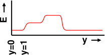
The second thing that we learn is that for any wave propagating at the required speed, the wavefunction can have any shape whatsoever, so long as it is differentiable function of its argument, i.e. a differentiable function of the phase Φ. It must be emphasized that we have not assumed that E is sinusoidal or even periodic. Any function E(Φ) you can think of, so long as it is differentiable, is an acceptable wavefunction for a plane wave in free space. Even an isolated blip, such as shown in figure 2, can be a solution to equation 58. The blip is moving left-to-right at the speed of light; the figure shows only a snapshot taken at time t=0.
The third thing we learn from equation 64 in conjunction with equation 63 is that once we have chosen E, then cB is constrained by equation 63. That is, at every point in spacetime, E = −kcB + g, where g is some constant of integration. This g is not very interesting. It is constant across all of space and time, and represents some uniform, non-propagating background field. It has no effect on the propagating wave; the wave just propagates past it.
This completes the task of finding some solution.
Let’s see if we can find a few more solutions.
First of all, we know the Maxwell equations are invariant under spacelike rotations, so we know there must exist plane waves propagating in any direction, not just the y direction. Any rotated version of our solution is another solution.
Secondly, you can easily verify that the factor of γ1 in equation 59 did not play any important role in the calculation; mostly it just went along for the ride. We could easily replace it with γ3 and thereby obtain another solution, propagating in the same direction as the previous solution, but linearly independent of it. This phenomenon is called polarization. The Ansatz in equation 59 is polarized in the γ1 direction. You can verify that the polarization vector must be transverse to the direction of propagation; otherwise equation 59 does not work as a solution to equation 58.
We won’t prove it, but we assert that we now have all the ingredients needed to construct the most general solution for plane waves in free space: first, pick a direction of propagation. Then choose a basis for the polarization vector, i.e. two unit vectors in the plane perpendicular to the direction of propagation. Then think of two arbitrary differentiable functions of phase, one for each component of the polarization vector. Finally, take arbitrary superpositions of all the above.
Tangential remark: Even though the Ansatz in equation 59 contains three terms, the fact that E=kcB and D=0 means it can be written as a single blade, i.e. a bivector that is the simply the product of two vectors. Specifically:
| (65) |
The structure here, and for any running plane wave, is simple. There are three factors: a scalar function E(Φ) that specifies the shape of the wave, times a spacelike vector that represents the polarization, times a null vector that represents the direction of propagation.
The general electromagnetic plane wave is not a single blade, but it can be written as a sum of blades of this form. Even more generally, there are lots of waves that are not plane waves.
As noted in section 11.1, there is a strict correspondence between the electric part and the magnetic part in an electromagnetic running plane wave. For a blip (or anything else) running left to right
| (66) |
This is sometimes expressed by saying the E field and the cB field are “in phase”. (Such an expression makes more sense for sinusoidal waves than for blips.)
Meanwhile, for a blip (or anything else) running right to left,
| (67) |
That is, once again there is a strict relationship between E and cB ... but the relationship in equation 67 is diametrically opposite to the relationship in equation 66. One of them is 180 degrees out of phase with the other.
If you consider the superposition of a left-running blip and a right-running blip, the whole notion of “phase relationship” goes out the window. You can have places where E is zero but cB is not, or vice versa, or anything you like, and the local relationship between E and cB will be wildly changing as a function of space and time. A particular type of superposition is considered in section 11.3.
A standing wave can be viewed as the superposition of equal-and-opposite running waves. In particular, let’s start with the sinusoidal waves
| (68) |
At any particular location y, the wave is a sinusoidal function of time. Choosing a different location just changes the phase. Let’s apply the trigonmetric sum-of-angles identity:
| (69) |
So, as advertised above, we see that at most locations – i.e. any location where cos(y) and sin(y) are both nonzero – the E-field and the B-field are 90 degrees out of phase for a standing wave. (They are in phase for a running wave, as discussed in section 11.2.)
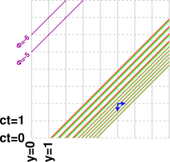
This section is restricted to the case where k=+1; that is, the wave is propagating in the +y direction. Also we assume the constant of integration g is zero. Therefore E = cB everywhere.
The blip we saw in figure 2 is portrayed again in figure 3. The former portrayed two variables, namely E versus y (at constant t). The latter portrays three variables, namely t, y, and E. The value of E is represented by the closeness of the flux lines. You can see that in the front half of the blip (larger y values) the E field is twice as large as in the back half of the blip.
The fact that E = cB corresponds to the fact that, at each and every point in spacetime, the number of flux lines per unit distance in the timelike direction is equal to the number of flux lines per unit distance in the spacelike direction. An example of this is portrayed by the two small blue arrows in the figure. Not only does each arrow cross the same number of flux lines, it crosses the same flux lines.
You can see that this is a direct consequence of the geometry of spacetime, and the fact that the wave is propagating with velocity v=c.
As shown by the purple lines, contours of constant phase run from southwest to northeast. Phase increases toward the south and east. Phase increasing to the south corresponds to temporal period, and phase increasing to the east corresponds to spatial period i.e. wavelength. Note that any attempt to measure period or wavelength is utterly frame-dependent. Some properties of the wave (such as the total number of cycles) are frame-independent, but other properties (such as period, frequency, wavelength, and wavenumber) are necessarily frame-dependent.
In figure 3, the x and z directions are not visible. If we made a more complicated diagram, from a different perspective, the electromagnetic field bivector F would be represented by tubes. The magnitude of F corresponds to the number of tubes per unit area.