|
| |
| Figure 1: Sinusoidal Motions in Spacetime | Figure 2: Density of Sources Near the Light Cone | |
The Liénard-Wiechert potentials are discussed in Feynman volume II section 21-5. If you have not re-read that section recently, I recommend you do so, but first let me offer a few words (and diagrams) that might clarify a couple of concepts.
Issue #1: Feynman writes an integral in equation 21.28, and writes a summation in equation 21.30 and in the unnumbered equation that follows. The implication is that the rest of the formulas in the chapter could be treated as integrands, to be integrated over all space.
This gets tricky because the main result, equation 21.34, involves a so-called «retarded time». If you want to know what fields are affecting the observer now, you have to know where the sources were at some earlier time. That’s simple enough for a source-particle that is not moving, or not moving very much. However, for a moving source-particle, the relevant time depends on position, and the relevant position depends on the time, so you wind up chasing your tail, unless you think about it just right.
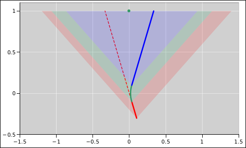
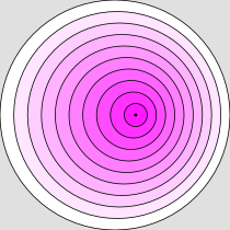
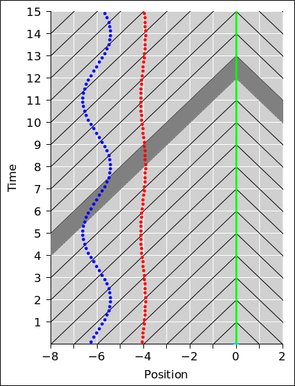
The smart thing to do is to integrate over all space and all time, subject to the restriction that the integrand lies along the observer’s light-cone. We can visualize what this means with the help of figure 1. For simplicity we show only one spatial dimension, plus the time dimension, so the light-cones look like diagonal lines, rather than full-fledged cones. These are shown in black in the figure. The observer is located at position x=0.
Physics tells us that as a general rule, in any given time interval, the observer is affected by the distribution of electrical charge and current in its past light-cone. For the interval from t=12 to t=13, the relevant region of spacetime is indicated by the gray-shaded band in figure 1. For a more mathematical way of expressing this, see section 1.2.
The spreadsheet used to produce these figures is cited in reference 1.
Issue #2: In figure 1, the red dots represent a charge that oscillates in the x-direction as a function of time, with a peak speed of 0.1 c. The blue dots are similar, except that the peak speed is faster, namely 0.6 c. The dots are equally spaced in time, according to the observer’s clocks. This is appropriate in terms of measure theory. That is, it means we can model the integral dt’ in equation 2b by counting dots.
In any given time interval, the number of red dots affecting the observer is very nearly constant, as you can see by counting dots between successive light-cones. For the blue dots, the story is much more interesting. Because of the spacetime geometry of the situation, when the particle is moving toward the observer, it spends significantly more time moving along (or nearly along) the light-cone. You can visualize this by counting the number of dots between consecutive black lines.
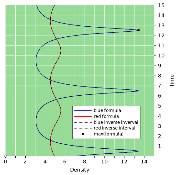
Note that figure 1 and figure 2 share the same time-axis. That means you can join the two figures together to make a 3D diagram. The density axis is perpendicular to the position axis, such that all of figure 2 lies within a contour of constant position x=0 when projected onto figure 1. The green background in figure 2 corresponds to the green vertical line in figure 1.
To say the same thing another way, the “time” used for plotting all curves in figure 2 is the time at which the field affects the observer, at the so-called field point, (t, r). You can see that the red curve in figure 2 peaks two seconds earlier than the blue curve; this is because the red source particle is two light-seconds closer to the observer. In contrast, in figure 1 the sources peak at the same time, as measured according to plain old time, relative to the observer’s contours of constant time.
Let’s be clear: The sloping black lines are contours of constant arrival time, while the horizontal white lines are contours of constant plain-old time (in the observer’s frame of reference).
The density of dots that affect the observer is plotted in figure 2. For today’s purposes, “density of dots” refers to the number of dots per unit time ... more specifically, per unit arrival time. A stationary particle would have 5 dots per second, at all times.
However, counting dots in an interval gives us only an average of the density over that interval. We would rather have something closer to an instantaneous estimate of the density. For this kind of discrete estimation, the shortest possible interval is the time between consecutive dots. The inverse of this interval is the density, i.e. dots per unit time. This is shown by the dashed black curves in figure 2. The peak density is about 13.5 dots per second, and occurs at time t=12.5. This is shown by a black dot in the diagram. The average density during the full second from t=12 to t=13 is somewhat less than the peak density. It is only 11 dots per second, as you can see by counting dots within the gray-shaded band in figure 1.
Of course in reality, the world-line source-point is not a series of dots, but rather a continuous curve. We can calculate the density directly, using the following formula:
| (1) |
Our discrete estimate (dashed black curves) differs from this formula (solid colored curves) by only about a percent at most, for the blue particle, under the given conditions. The discrepancy is much less for the red particle.
Equation 1 comes directly from the geometry of the situation as shown in figure 1. It is the same equation you would get for the intersection of sloping lines. At location (t,x) = (3.5, −6) the two lines are sloping in opposite directions, so they meet in roughly half the time it would take for either one to hit a stationary vertical line. Later, at location (t,x) = (12.5, −6) the two lines are sloping in the same general direction, so it takes a long time for the steeper line to catch up. (If you flip the diagrams so that time is horizontal and position is vertical, it becomes even easier to interpret slope as velocity.)
In equation 1, the 1 in the denominator comes from the slope of the light-cone, while the v/c comes from the slope of the world-line of the particle. It’s just geometry.
In this section, we assume the current density (including charge density) is known a priori.
Recall that we dealt with issue #1 by integrating over all space and all time, subject to the requirement that the integrand lies along the observer’s light-cone. Mathematically, this requirement can be expressed by a Dirac delta-function, so that the Liénard-Wiechert potentials take the form:
|
where r is the field point, i.e. the place where we are evaluating the field, and r′ is the source point, i.e. the location where the current density (including charge density) resides.
Feynman did not write the potentials in the form equation 2. He avoided delta functions completely. Undoubtedly he knew about delta functions, but presumably he was trying to do the students a favor by not mentioning them. It is entirely possible that the students, at this point in their education, had never seen delta functions. Feynman did warn us near the end of section 21-1 that some “gory details” would get swept under the rug.
According to the modern (post-1908) understanding of the subject, we take J to be a four-vector. The timelike component of the current is the charge density, in the appropriate units:
| (3) |
See section 4.3 for more about this.
We are tempted to do the same thing with the vector potential. We can define a potential with four components:
However, beware that even though A looks like a four-vector, it isn’t really. It behaves “almost” like a four-vector, but not quite. For details on this, see section 4.2.
Even though it is a bit of a swindle, there is some mnemonic value in writing things in a way that shows the correspondence between ϕ and the spacelike part of A. We can make the correspondence more apparent if we make it a habit to write things in terms of cρ and ϕ/c (rather than plain ρ and ϕ). For details on this, see section 4.3. In any case, keep in mind that we are treating r and r′ as three-dimensional vectors. That gives us:
|
Equation 5 tells us that the field at (t, r) depends on what the source was doing at some earlier time at some far-away point (t′, r′). The times and positions must satisfy the light-cone condition:
which is, alas, not a closed-form expression, since t′ appears on both sides of the equation. Even if we know the source position r′ as a function of time, it is not easy to obtain an explicit equation for t′ (except in trivial cases, such as a stationary source). On the other hand, equation 6 does have a clear meaning, as you can see in figure 1: If the point (t′, r′) lies on the light cone, it contributes; otherwise, it doesn’t. For outgoing waves, we care about the past light-cone only. We expect the world-line of the source particle to cross the past light-cone only once, so equation 6 has a unique solution. If need be, you can find the solution (to a high degree of approximation) using a binary search.
The four-dimensional delta function in equation 2 captures the light-cone idea. It makes everything nice and symmetric, and treats r and t on the same footing, to the extent possible.
Another way of looking at things starts with a change of variable. Let s be the separation vector from the observer to some source-point. The absolute position of the observer is r so the absolute position of the source is r+s. Contours of constant |s| are shells surrounding the observer. Integrating over all s is the same as integrating over all space, just with a different way of looking at it.
|
The last two lines are synonymous with the solutions Feynman wrote in the bold black box at the end of section 21-3. Again, beware that [ϕ, A] is not a 4-vector.
We now return to issue #2. We consider the special case where the field is associated with a single point charge. That means that all four components of J (including ρ) are delta functions. They’re three-dimensional delta functions. Let w(t) be the world-line of the particle. The current density is
where q is the charge of the particle.
Equation 8 tells us there is current density (including charge density) along the world-line of the particle and nowhere else. When we stick that into equation 2, we get a four-dimensional integral with four delta functions multiplied together in the integrand.
|
We can do the integral over r′ immediately. That leaves us with:
|
When doing the integral over t′ we have to be careful. Whenever you integrate something where the argument of the delta function is itself a function, it pulls out a factor of the derivative of the argument, as discussed in section 4. This gives us another way of understanding the density factor expressed by equation 1.
|
where on the RHS the primed quantities (t′, w(t′), and v(t′)) pertain to a source point that satisfies the light-cone condition, equation 6.
We can rewrite the equation in a form that is perhaps easier to interpret:
|
Here is yet another way to rewrite the equation:
|
where U is a unit vector in the direction from the source point to the field point. This form is in some ways easier to understand, but in some ways easier to misunderstand. Beware that U is an odd duck, insofar as it depends on both the field point (t, r) and the source point (t′, r′). In particular, because of U, you cannot look at the equation and assume that all unprimed quantities are independent of the source point.
The middle factor on the RHS of equation 11a, equation 11b, equation 13a, or equation 13b is a generalization of the density factor we saw in equation 1, generalized to handle motion in more than one dimension. If the source velocity is non-relativistic (or if the source motion is perpendicular to the line of sight) this factor drops out.
Here’s another way of writing the potentials. This is compact and convenient for calculations.
|
Note that as the speed |v| approaches the speed of light, if the source charge is moving toward the observer, the density factor in equation 1 becomes enormous. In other words, a relativistic oscillator radiates like crazy. In particular, suppose you have two oscillators with the same dipole moment and the same frequency of oscillation. One consists of a large charge moving at low speed, while the other consists of a small charge moving at high speed. If the high speed is near the speed of light, the high-speed oscillator will radiate vastly more than the other oscillator.
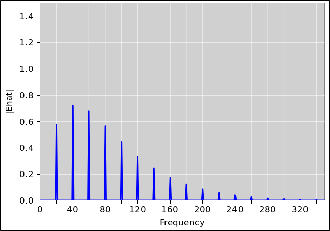
Also note that the blue and cyan curves in figure 2 are nowhere near being sine waves. The frequency of the radiated light will not be confined to the frequency of oscillation; higher harmonics will be present in abundance. Figure 3 shows the spectrum for a source undergoing purely sinusoidal motion. The source has a frequency of 20, and a peak velocity of 0.9 c.
This example illustrates – yet again – the idea that when faced with any situation involving space and time, the first step should be to draw the spacetime diagram. Many things that would otherwise be very mysterious have a simple geometrical interpretation. If you can represent the situation on a spacetime diagram, the geometry becomes much easier to visualize.
Spacetime diagrams are famously useful for special relativity. Keep in mind that special relativity is nothing more (or less) than the geometry and trigonometry of spacetime, as explained in reference 2. “Standard” relativity problems tend to involve factors of √(1−v2/c2). The Liénard-Wiechert density factor involves a different factor, namely 1−v/c. However, it’s still a spacetime geometry problem, and it still helps enormously to draw the spacetime diagram.
Here’s something that’s fun to think about. Consider the contrast:
The question arises, can we obtain a consistent view of these two facts? This is not going to be easy, because starting with the 1/r2 Coulomb field of a point charge, I don’t see any way to explain the 1/r radiation field. By way of contrast, if there is some sort of cancellation, I can arrange something that falls off faster than 1/r2 – such as a dipole field that falls off like 1/r3 – but I cannot cook up anything that falls of slower than 1/r2. I’ve seen a number of books that claim to explain things this way, but it never made any sense to me.
So some profound questions remain:
The short answers are (a) no, (b) no, and (c) yes.
The only way to explain the two behaviors is to realize that there are two different contributions to the field, one of which is dominant at short distances and long times, while the other is dominant at long distances and high frequencies.
Let’s write the Maxwell equations in modern, four-dimensional form. For details on this, see reference 3.
| ∇ F = |
| J (15) |
The ∇ operator on the LHS generates a large number of terms, and it turns out that different terms are needed to explain the Coulomb field and the radiation field. However, rather than pursuing the mathematics, let’s try to get a qualitative understanding.
The easiest way to get a unified view of what’s going on is by considering the potentials, namely the vector potential and the scalar potential. For a nonmoving point source, we get a scalar potential that falls off like 1/r, as you can see from the Liénard-Wiechert formulas, such as equation 13b.
As usual, it pays to think in four dimensions. We can construct a four-vector-ish quantity A. The timelike part of A is the scalar potential (commonly denoted ϕ), while the spacelike part of A is the three-dimensional vector potential.
The electromagnetic field bivector is then given by the following equation, which implicitly defines what we mean by A:
| (16) |
So now we can ask, given that the radiation field falls off like 1/r, why can’t the static electric and static magnetic fields do the same? Why do the static fields have to fall off like 1/r2?
Well, there are several reasons. In all cases, keep in mind that the piece of F that we call the “electric” field is the timelike component of F. Also keep in mind that the potential A falls off like 1/r. Let’s consider the various cases one by one:
Note that the spatial derivatives of A have a 1/r2 dependence, while the time derivatives have a 1/r dependence. We can summarize the situation as follows:
| d/dt | d/dx | |||
| source=charge: | 0 | 1/r2 electric | ||
| source=current: | ω/r radiation | 1/r2 magnetic |
Starting from a point charge (or a dipole), we can cobble up a field that goes like 1/r by taking two time derivatives: The first derivative gives us a current, which contributes to the spatial part of A in accordance with equation 13a. The second time derivative gives us the electric field in accordance with equation 16.
To repeat: Yes, we can have an E-field that goes like 1/r, but it requires taking either one time-derivative of the current or two time-derivatives of the point-charge potential. We recognize this as the radiation field.
Conversely, if we want a static E field, we need to take a spatial derivative of the point-charge potential, and that gives us something that falls off like 1/r2. We recognize this as the Coulomb field.
As discussed in section 3.1, it is not possible to simply wiggle the Coulomb field and thereby produce the radiation field. There are calculations you can do that are more-or-less correct that look Coulombic but really aren’t. (Either they’re not correct or not Coulombic.)
Here’s a fun fact: For a charge moving at a uniform velocity, all the electric field lines point directly at the charge.
In more detail: To zeroth order, the charge drags the whole pattern of electric field lines along with it. That is true even far from the charge, which is quite remarkable. Think about it: At the current time t, relativistic causality tells us that the field lines at a distance cΔt from the charge don’t really know where the charge is now; they only know where it was at the previous time t−Δt. The trick is that the field can predict where the charge is going to be, based on what it was doing at the earlier time, assuming it will continue its uniform straight-line motion.
To a first order, a moving charge creates a magnetic field to go along with the electric field. To second order, the intensity of the electric field is modified (but the lines still point to the charge).
For a charge that undergoes a period of acceleration, the field lines point to the predicted location of the charge; that is, the location (at the relevant retarded time) where it would have been if there had been no acceleration.
Here is a diagram slightly modified from reference 4.
Figure 4 shows the spacetime diagram for a charged particle that bounces. Specifically: It starts out moving right-to-left at a uniform velocity v = −v0 (as represented by the red line), then undergoes a brief period of uniform proper acceleration (green), and thereafter moves left-to-right at uniform velocity v = +v0 (blue). The red dashed line indicates what would have happened if it hadn’t bounced, and instead just maintained the initial velocity. The total change in velocity is Δv = 2v0.
The extrapolated red line and the extrapolated blue line cross at the origin. If you look closely, you will see that the actual trajectory does not quite go through the origin, because the bounce pushes it away before it gets there. Imagine some sort of force field acting on the particle.
The acceleration is a constant proper acceleration. That is to say, it is constant when measured in a series of frames instantaneously comoving with the particle. Therefore this part of the worldline is a hyperbola, as seen in the lab frame. (When Δv is small compared to c, the hyperbola is indistinguishable from a parabola, but the hyperbola is the more general, more reliable answer.)
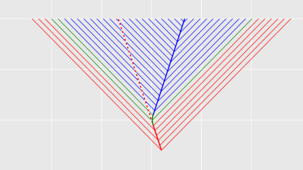
Figure 5 is another depiction of the same situation. Instead of shading, it shows null (light-like) rays radiating away from the worldline of the particle.
Note that in the blue part of the diagram, there are exactly twice as many rays per unit time on the left side (behind the moving particle) as there are on the right side (ahead of the moving particle). [The speed (|v0| = c/3) was chosen to make this a round number.]
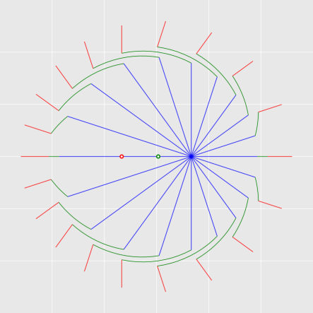
The corresponding field line diagram is shown in figure 6. Everything in this diagram pertains to the present time, i.e. now, i.e. t=1. The bounce occured in the past, at t=0. The red-shaded cone indicates the region in spacetime where the Liénard-Wiechert potentials are derived from the red part of the particle’s world-line. Similar words apply to the green-shaded and blue-shaded cones.
The top of figure 4 (i.e. t=1) corresponds to the horizontal midline of figure 6.
This is vaguely reminiscent of the sacred I’itoi symbol (The Man in the Maze).
The green dot marks the center of the world, in the lab frame.
Figure 6 does not represent a particle that moved from the red point to the blue point. The diagram is a snapshot taken at the present time (t=1). There is nothing at the red point; it is where the particle hypothetically would have been if it hadn’t bounced.
The shell that divides the inner and outer parts of the diagram is shown in green. It is centered in the lab frame, i.e. centered in the lab frame. The shell is thin because the bounce was rather sudden and impulsive. It occurred over a short time Δt.
As a consequence the green shell maintains a constant thickness c Δt, constant over time as the radiation moves outward. It depends only on how suddenly the bounce occurred.
The green links that connect the blue lines to the red lines get longer over time. Their length is proportional to t Δv or equivalently r Δv/c. That is, their length depends on how long it has been since the bounce (not how suddenly the bounce occurred). This means the radiation field is a factor of r stronger than the Coulomb field. It decreases like 1/r not 1/r2.
The previous two paragraphs tell us the radiation field is transverse in the far field. (It’s a mess in the near field.)
This diagram gives a rough idea of what’s going on, but it cannot possibly be exactly right, for various reasons:
We know the red lines and the blue lines are correct, but simply joining them up by drawing green links is not well founded in the fundamental equations. In particular, the sharp corners when the connections occur require there to be a ton of curl in this region. This would require more-or-less infinite magnetic fields in these regions.
In particular, once you decide that we are going to have nonzero curl in the transition region, you can add closed loops of E ... and it will take some very fancy hand-waving to convince me that the number of closed loops shown in the diagram (i.e. zero) is correct.
Keep in mind that you cannot understand this in Coulomb-only terms.
Figure 7 shows the Coulomb potential for a charge in uniform straight-line motion. No acceleration. You can see that the electric field, i.e. the gradient of the potential, does not point toward the present location of the charge. This is particularly clear along the 12:00 – 6:00 axis of the diagram.
The figure is not wrong as far as it goes, but is incomplete and therefore misleading. To get the right answer, you would have to use the full four-vector-ish potential (suitably retarded). When you differentiate the full four-vector-ish potential to find the field lines, you get the predictive behavior described above.
Let’s be clear: You cannot explain the field of an unaccelerated charge in terms of Coulomb’s law, much less an accelerated charge.
An unaccelerated particle drags the potentials along. The potentials are retarded, as required by relativistic causality.
The particle also drags the electric field pattern along. The fields look like they are not retarded, but really they are retarded with a prediction. Coulomb’s law does not contain the prediction terms; you need the full four-vector-ish potential for that.
Also keep in mind that electric field lines are not real. The E and B lines are an approximate model, nothing more. In particular, this situation, requiring a near 90 degree bend in the field lines, is the sort of thing that is very likely to break the model. You can do somewhat better by looking at the electromagnetic bivector.
Constructive suggestion: Whenever you see a reference to «retarded time», don’t take it literally. Replace it with the light-cone condition, equation 6. If the source point is on the light cone it contributes; otherwise it doesn’t.
Here’s a copy of equation 4. We can define a potential with four components:
| (17) |
Beware that A is not quite a 4-vector. It does not behave properly under Lorentz transformations. Loosely speaking, if you start out with a vector potential in a certain gauge and then change to a different reference frame, you get a vector potential with the same physical meaning in some other screwy gauge. If you try to calculate A by evaluating it in one frame and then boosting it into another frame, you will almost certainly get the wrong value for A.
However, this is not tragic, because the potentials are not directly observable. When you compute any physical observable, the gauge drops out, so you should end up with the right physics. The only thing that matters to the physics is the difference between two potentials, and that turns out to be well behaved. In particular, the key equation is OK:
| (18) |
The electromagnetic field F is a well-behaved bivector. The exterior derivative on the RHS annihilates any and all gauge fields.
At some sufficiently-vague conceptual level, the problems with A don’t matter ... but if you’re doing actual calculations, sometimes they do matter.
In any case, we can make the problems go away by defining a new equivalence relation. Suppose we have two potentials A1 and A2. We say that A1 is equivalent to A2 modulo a gauge and write A1 ∼ A2 if-and-only-if they differ by a gauge field, i.e. if ∇∧(A1 − A2) = 0. You can verify that this is a legitimate equivalence relation, i.e. that it is reflexive, symmetric, and transitive. If A1 ∼ A2, we can’t assume they are “equal” because they are not necessarily equal in the component-by-component sense ... but they are equivalent modulo a gauge, and they represent the same physics.
We can achieve a similar result by defining an equivalence class: Let Ã1 be the set of all potentials that differ from A1 by a gauge. The set Ã1 is closed under gauge transformations. We can then write Ã1 = Ã2, because the two sets contain exactly the same elements.
Consider the four-velocity of a particle: In spacetime, in its own rest frame, it is moving toward the future at a rate of 60 minutes per hour. Meanwhile, the three spacelike components of the four-velocity are zero.
We can use this idea to understand the current density as given by equation 3. The timelike component of J is cρ. That represents a current in spacetime, flowing toward the future.
Similarly, the factor of c that appears on the RHS of equation 8b is related to the fact that the v that appears in equation 8 is the so-called coordinate velocity, i.e. the reduced velocity, i.e. the derivative of the four-dimensional radius vector x with respect to coordinate time t:
| (19) |
The reduced velocity is not to be confused with the four-velocity, which is the derivative with respect to the proper time τ:
| (20) |
The zeroth component of the radius vector is x0 = ct, so the zeroth component of the reduced velocity is simply c:
| (21) |
Whenever you integrate something where the argument of the delta function is itself a function, it pulls out a factor of the derivative of the argument. Specifically:
| (22) |
where x0 is a root of the function g(); that is, g(x0) = 0. The “⋯” indicates that there is one term for each root. However, for the case of outgoing waves from a point charge, there is only one root that we care about. (For incoming waves impinging on an absorber, there would be another root, somewhere on the forward light-cone.) You can easily verify equation 22 by doing a change of variable in the integral.
To get from equation 10 to equation 11, we need the following derivative:
|
Beware that even though it is usually better to work in four dimensions, we are treating r and w(t′) as three-dimensional vectors, and the dot product in equation 23c is a three-dimensional dot product.
If you can make use of .xls files but not .gnumeric files, you can
see how far you get with this:
./lienard-wiechert.xls