Figure 1: Four Wedges
You probably learned all five of those things separately.
Now suppose that you could learn one simple theory that explains all five of those things together. It shows that those five things are mutually consistent and not exceptional ... including the low-speed limit, the high-speed limit, and everything in between. It explains all that and lots more besides.
Well, we have such a theory. It’s called special relativity. It gives a unified understanding of many things that would otherwise have to be learned separately.
Most remarkably, it does all of this using only one tool: non-Euclidean geometry and trigonometry.
Note: Many of the expressions in this section have been written in scare quotes «...», because they are valid only in the non-relativistic approximation. They should not be taken as gospel. In particular, the non-relativistic «p» used here must not be confused with the spacetime vector p used in the rest of this document. The latter is much more useful.
Applying the ideas of special relativity is more interesting than deriving them. The goal is to get to some applications as soon as possible, but first let’s briefly mention a couple of fundamental principles.
If you are interested in a more deductive approach, see reference 1 and reference 2.
This is Galileo’s principle of relativity. It says that if you shut yourself up in a room in a ship, you cannot tell the difference between a stationary ship and a ship that is undergoing uniform straight-line motion ... assuming you are truly isolated from any outside influences. For a fuller statement of this principle, see section 6.1.
The laws of physics are invariant with respect to rotation. That is, if you shut yourself up in a room in a ship, you cannot tell which direction is which ... assuming you are truly isolated from any outside influences.
The laws of physics depend only on what is happening in the immediate neighborhood of here and now. That is to say, they do not depend on far-distant places or far-distant times.
We start by giving the position vector an “extra” dimension, but that is just the beginning. Given this new notion of position, it should come as no surprise that the velocity, acceleration, and momentum also have an “extra” dimension.
Vectors in spacetime are sometimes called “four-vectors” but that is unnecessarily complicated. It is better to call them simply spacetime vectors. Often there are only two dimensions that matter. For example, for relativistic motion in a straight line, it suffices to understand the tx plane. We can draw nice two-dimensional pictures of that. Even when there are more than two dimensions involved, it is often possible to visualize them two at a time. (We postpone higher-dimensional stuff to section 5.)
This is important, because most people – even professional physicists – have a hard time visualizing rotations in three dimensions, let alone four.
People like to say that time is the fourth dimension, but that’s misleading for multiple reasons. For one thing, it’s inconsistent with the idea of two-dimensional spacetime, e.g. the tx plane, as discussed in the previous paragraph. Perhaps more importantly, it doesn’t make sense for anything except position vectors. Whereas the “extra” component of the position vector is called the time, the “extra” component of the momentum vector is called the energy. We can summarize this as follows:
| (1) | ||||||||||||||||||||||||||||
In the previous equation, we have chosen to measure things in units such that the speed of light comes out to be c=1. More generally, we can stick in the factors of c explicitly:
| (2) | ||||||||||||||||||||||||||||
If you are wondering why the timelike component of the position involves a factor of c, while the timelike component of the momentum involves a factor of 1/c, don’t worry about it too much. There are no fundamental issues here.
We could discuss this in terms of t and x, but it is just as easy (and more informative) to discuss t, x, y, and z together:
| In three dimensions, in any particular reference frame, we can always construct three basis vectors x̂, ŷ, and ẑ. | In four dimensions, in any particular reference frame, we can always construct four basis vectors t̂, x̂, ŷ, and ẑ. |
These three vectors are normalized as follows:
|
These four vectors are normalized as follows:
|
The minus sign that appears in equation 4a is the only thing that makes spacetime different from ordinary Euclidean space. Surely you already knew that the time dimension is not exactly the same as the spatial dimensions. Now you know exactly how different it is ... and also how similar it is.
The basis vectors are of course
mutually orthogonal:
|
The basis vectors are of course mutually orthogonal:
|
Note: It is possible to deduce all of special relativity using just the two big ideas presented here. We’re not going to take a purely deductive approach, but we could if we wanted to.
At this point, we already know enough special relativity to do some interesting things.
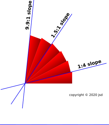
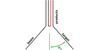
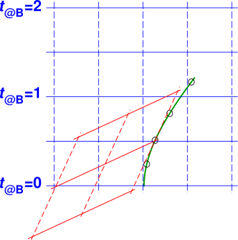
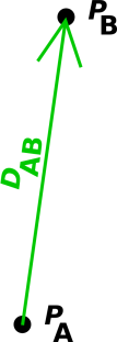
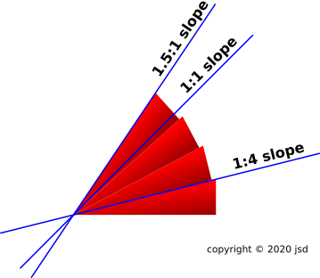
Suppose we have four wooden wedges, each with a slope of 1:4, i.e. a rise of 1 for each run of 4. That corresponds to an angle of about 14∘. Let’s stack up four of them with their tips together, as shown in figure 1. The angles add as you would expect, so the combined angle is 56∘. However, the behavior of the slope is not so simple. The combined slope is not four times as large. It is not 1:1. In fact it is nearly 1.5:1. When the angle goes up by a factor of 4, the slope goes up by a factor of 6.
We can play the same game with six wedges, as shown in figure 2. When the angle goes up by a factor of 6, the slope goes up by a factor of 39½.
Suppose we have Particle A moving to the left (relative to the lab frame) at 80% of the speed of light, and Particle B moving to the right, also at 80% of the speed of light. How fast are they moving apart, relative to each other?
The answer is not 180
We can find the right answer by using the ideas of section 4.1.
| Slope is a ratio in the xy plane, namely the ratio of y to x. | Velocity is a ratio in the tx plane, namely the ratio of x to t. |
In Euclidean space, the angle is tan(y/x). In particular,
for the six wedges:
|
In
spacetime, the angle is tanh(x/t), using the hyperbolic tangent.
In particular, for our example:
|
| In Euclidean space, adding the angles (if they are not too large) always gives you more slope than you would get by naïvely adding the slopes. | In spacetime, adding the angles always gives you less speed than you would get by naïvely adding the speeds. |
Just to be clear: Particle A is moving away from Particle B at 97½% of the speed of light. This is easy to understand in terms of the geometry and trigonometry of spacetime.
For a more advanced application of this idea, see section 4.19.
In this section, we will show how the famous formula for kinetic energy, KE = ½ m v2, can be understood as a consequence of special relativity, i.e. as an approximation, valid in the low-speed limit. We will also derive some better approximations, notably KE = ½ p·v.
Suppose we have a particle moving through space. As a first application, let’s investigate it’s momentum and energy.
The object exists as a thing unto itself, independent of whatever coordinate system, if any, we choose. This is analogous to the ruler in figure 3. There is nothing remarkable about this.
What’s more remarkable is that the energy and momentum can be described by a vector, and this vector also exists as a physics entity unto itself, independent of whatever coordinate system, if any, we choose. This may require some explaining.
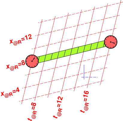
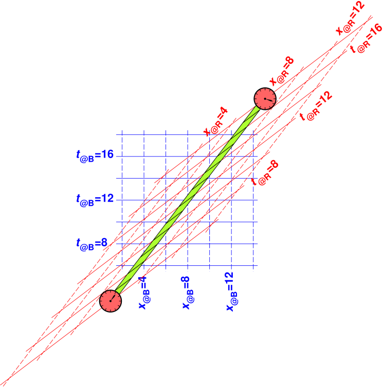
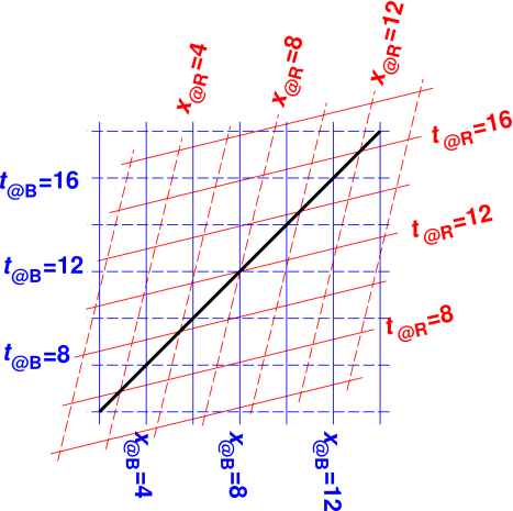
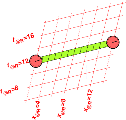
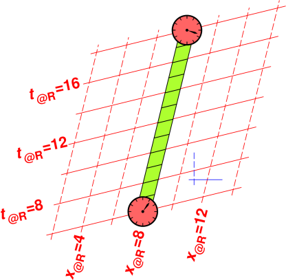
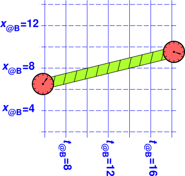
Let’s choose a reference frame, called the red reference frame. We arrange it so the particle has no x- y- or z-velocity measured using this frame. This is the situation shown in figure 4. The green bar is not a ruler, but rather the track of a small particle moving through spacetime. The particle is located at x=8. It just sits in one place and gets later.
Now that we have a coordinate system, we can write the particle’s position vector in terms of components, namely [t, x, y, z]@R. The spacetime velocity u is the rate-of-change of position with respect to proper time, τ. (Proper time is the time as measured by a clock comoving with the particle.) In this situation, τ is identical to the t@R component. When calculated using the red reference system, the spacetime velocity is:
| (9) |
This is particularly simple because in the red reference frame, the x, y, and z components of position are unchanging, and dt/dτ=1. That is to say, in a frame where the particle is at rest, the t-component is the same as proper time.
Compare equation 71.
It must be emphasized that the spacetime velocity is never zero. This may seem odd, but it turns out to be useful. For one thing, it makes the statement of various conservation laws much more elegant; see reference 3. For another, it permits a consistent view of velocity, momentum, and energy (including rest energy) as discussed in section 4.6.
Let’s be clear: When we say a particle is “at rest” in a given coordinate system, it means the x, y, and z components of its velocity are zero. The spacetime velocity as whole is never zero. When “at rest”, the particle is moving toward the future at a rate of 60 minutes per hour.
If we stick in the explicit factors of c, we find u = [c, 0, 0, 0]@R.
The spacetime momentum could hardly be simpler. It is just the mass times the spacetime velocity:
| (10) |
In all cases, we define the gorm of a vector to be the dot product of the vector with itself. It has the following properties:
| In Old-fashioned Euclidean Space | In Spacetime |
| For a vector with components x, y, and z, the gorm is equal to x2 + y2 + z2. | For a vector with components t, x, y, and z, the gorm is equal to −t2 + x2 + y2 + z2, with an important minus sign in front of the t2 term. The minus sign is necessary. It is an inescapable consequence of the minus sign in equation 4a. |
| The gorm is always positive or zero. It is the square of the «norm». | The gorm might be negative, so it cannot be expressed as the «norm» squared, or any other scalar squared. Indeed the whole idea of «norm» is dead on arrival. Complex numbers don’t help. For a great many purposes, we can rely on the gorm, without trying to take the square root thereof. |
| For a vector V, we can write the «norm» as |V| and the gorm as V·V or equivalently V2, which happens to be the same as |V|2. | For a vector V, we do not write |V| or |V|2. That would make sense for a result that was always positive, but we cannot assume that. The gorm is simply V·V or equivalently V2. |
| The gorm is the square of the length. | If the gorm happens to be positive, we say the vector is spacelike. In this case, we can interpret the gorm as the square of a proper length. |
| If the gorm happens to be negative, we say the vector is timelike. In this case, we can interpret the gorm as the negative of the square of a proper time. The minus sign is necessary. |
| If the gorm of a vector is zero, the vector is zero. If you choose a basis, every component of the vector is zero. | If the gorm is zero, the vector might or might not be zero. If the vector is nonzero but its gorm is zero, we say the vector is lightlike. For example, a vector with components [t, x] = [1, 1] has gorm=0, even though the components are nonzero. For details, including a diagram, see section 4.16. |
| The gorm is unchanged by rotations. | The gorm is unchanged by rotations. Indeed, it is unchanged by timelike rotations (i.e. boosts) as well as old-fashioned spacelike rotations. |
As always, if we know how to calculate dot products involving the basis vectors, as in equation 4 and equation 6, we can calculate any dot product whatsoever. Just expand each vector as a linear combination of basis vectors, take the dot product, and turn the crank. All of the aformentioned properties of the gorm can be verified in this way. On the other hand, all the important properties of vectors can be expressed without reference to any basis. The vectors are physical objects unto themselves, independent of whatever basis (if any) you choose.
Without mentioning any basis, we can say that the gorm of the spacetime velocity (u) and spacetime momentum (p) are always:
| (11) |
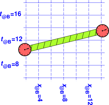
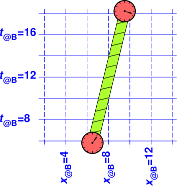
That is obvious when using the basis derived from the red coordinate system. We can learn something by evaluating the same two gorms using another basis, namely the one derived from the blue coordinate system shown in figure 5.
We know from equation 1 that p = [E, px, py, pz]@B. When we calculate the gorm in terms of these components, we find it is equal to − E2 + px2 + py2 + pz2. Meanwhile, the gorm is still equal −m2. We know this because we calculated it using the red coordinate system, and we know that the gorm is invariant with respect to rotations. Combining these two expressions for the gorm, we obtain:
| (12) |
We can re-arrange that to obtain a result that is not an elegant spacetime result, but is interesting because it makes contact with the pre-1908 way of looking at things, expressing the energy as a function of the spacelike part of the momentum:
| (13) |
On the last line we have stuck in the explicit factors of c.
We can simplify the equations by introducing the 3-momentum, pxyz. In any particular reference frame, it is just the spatial part of the spacetime momentum. That is:
| (14) |
Combining equation 14 with equation 13, we can write:
| (15) |
On the last line, we have stuck in the explicit factors of c. As always, pxyz2 is shorthand for the dot product pxyz·pxyz.
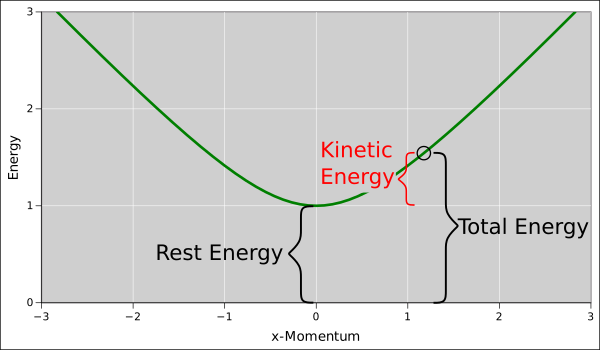
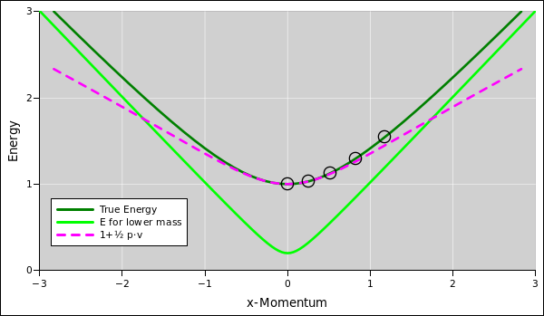
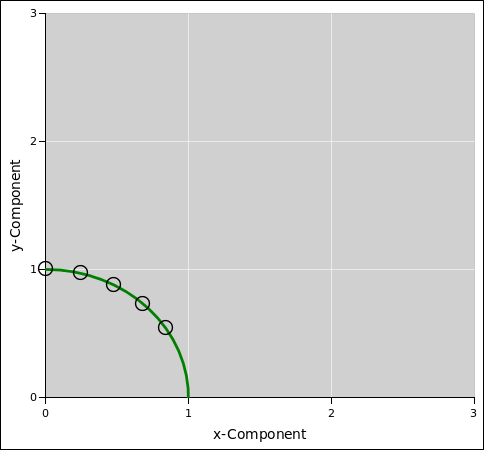
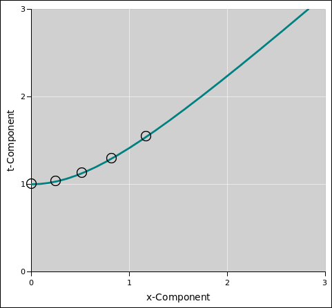
Let’s examine equation 15 more closely. The first thing to do is to draw the graph of E versus pxyz. It’s a hyperbola. Figure 6 shows the case where m=1 and c=1. For simplicity, the graph assumes the 3-momentum has no y or z components. (We can always rotate our point of view to make this happen.) The small black circle in figure 6 represents 1 radian. Note that 1 radian corresponds to a reduced velocity (v) equal to 76% of the speed of light.
One thing that we notice immediately is that the energy is equal to mc2 when the particle is at rest and not otherwise. Let’s be clear: The famous equation E=mc2 is very widely misunderstood. It would be better to rewrite it to emphasize that mc2 corresponds to only part of the energy, namely:
| (16) |
This E0 is more-or-less universally called the rest energy.
| This makes perfect sense for particles that have nonzero mass. When the particle is at rest, its total energy E is equal to the rest energy E0. | For a massless particle such as a photon, calling E0 the “rest energy” is a bit of a misnomer. A running-wave photon has a well defined mass, namely m=0 which means E0=0. However, strictly speaking, we ought not call this the rest energy because the photon is never at rest. Its total energy E is never equal to E0. |
| This is mostly a minor terminology issue when discussing massless particles; it is rarely if ever a serious problem. See section 4.26 and section 4.28 for some related discussion. |
Actually, we hardly need a name for E0 at all. Since we are using equation 16 to define E0, the equation is automatically and tautologically true. I don’t want to get into a metaphysical argument over whether E0 «is» the mass; all that matters is that it is numerically equal to the mass, when mass is measured in energy units. If we used sensible units, measuring distance in the spacelike directions using the same units we use for the timelike direction, then c would be equal to 1, and energy units would be the same as mass units.
Because it is a tautology, equation 16 is not terribly interesting. We are far more interested in equation 15, which tells us how E0 (the rest energy, aka mass) is related to E (the plain old total energy).
One should never say that mass is “equivalent” to energy, because “equivalent” is much too strong a word. An equivalence relation is reflexive, symmetric, and transitive; for details see reference 4. One would not say that Lake Baikal is equivalent to water, because some of the world’s water is in Lake Baikal but some is not. By the same token, one should never say that mass is equivalent to energy, because some of the the world’s energy is in the form of mass but some is not.
If you want to say mass corresponds to a subset of the energy, that’s fine, in accordance with equation 16. Just don’t leave out the word “subset”. For any single particle, the total energy E (in your chosen frame) is equal to the rest energy mc2 if and only if the particle is at rest (in that frame). The case of multiple particles is discussed in section 4.26 and section 4.28.
When the particle is moving slowly, we can learn some amusing things by expanding equation 13 to lowest order. In any given frame, we have:
| (17) |
As shown in figure 6, we define the kinetic energy (in the given frame) to be everything except the rest energy:
| (18) |
That formula is algebraically correct, but is numerically badly behaved in the non-relativistic limit, when the kinetic energy is tiny compared to the rest energy. Equation 19b is equivalent algebraically, and much better-behaved numerically, as discussed in reference 5. A more detailed discussion of spacetime kinetic energy, including the numerical-methods issues, can be found in reference 6.
|
You can easily show the two forms are algebraically equivalent. Hint: divide one by the other.
Equation 18 and equation 19 are valid at all speeds: fast, slow, and in between. In the low-speed limit, we can approximate the kinetic energy using a Taylor series:
|
It is well known in classical physics that the kinetic energy is ½pxyz2/m. Special relativity is telling us that classical physics can be considered a lowest-order approximation to the true spacetime physics.
| |
There are other ways of expressing this result, some of which will turn out to be useful later. To proceed, we need to introduce the classical velocity v, which is purely spacelike, so v = vxyz. For present purposes, it suffices to note that pxyz is the classical momentum, and the classical velocity v is approximately equal to pxyz/m for a slow-moving particle. As discussed in section 4.5, this is not the official definition of v, but it is a good approximation at low speeds, which is the regime we are considering.
| (21) |
The approximation pxyz ≈ mv is an excellent approximation for a slowly-moving particle. It is correct to first order, and indeed to second order, as discussed in section 4.5.
We can interpret equation 21 as saying that the particle has a kinetic energy of ½ pxyz·v, plus a non-kinetic energy (rest energy) of mc2. The kinetic energy depends on the 3-momentum, while the rest energy does not. This is not the elegant spacetime way of looking at things, but it shows how relativity reproduces the classical pre-1908 ideas.
Now let’s consider the opposite extreme, namely photons or other particles that have little or no mass and/or very large momentum, such that the momentum terms dominate on the RHS of equation 13. We see immediately that in this limit
| (22) |
| For a fast-moving massive particle, these expressions are true to a good approximation. We have used the fact that the particle’s speed is very nearly the speed of light. | For a massless particle such as a photon, these expressions are exact. The particle’s speed is equal to the speed of light. |
Comparing equation 22 with equation 21 is interesting. We see that the slow-moving particle has a kinetic energy equal to a half pxyz·v, whereas the fast-moving particle has a kinetic energy equal to a whole pxyz·v. This may seem peculiar, but it is in fact correct.
The nice thing about special relativity is that it allows us to simultaneously understand the slow-moving particles and the fast-moving particles and everything in between. In particular:
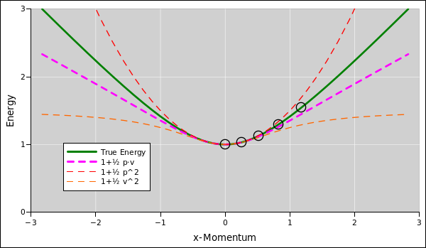
Figure 7 is similar to figure 6, but with some additional detail. The dark green curve, as before, represents the case where m=1, while the light green curve represents a less-massive particle, m=0.2.
You can see that:
The small black circles in figure 7 indicate different rotation angles in the tx plane, from 0 to 1 radian in steps of 1/4 radian.
The dashed magenta curve in figure 7 represents the recommended approximation presented in equation 21, namely E≈mc2+½pxyz·v. You can see that it is a very good approximation at moderate speeds, and even at the highest speeds it is never off by more than a factor of 2.
The other approximations presented in equation 21 are just as good when the speed is small, but not otherwise. At high speeds, E≈mc2+½pxyz2/m is a woeful overestimate, while E≈mc2+½mv2 is a woeful underestimate. This is shown in figure 8.
Figure 7 is in some ways related to figure 5. The relationship becomes more clear if we transpose figure 5, so that x increases horizontally and time increases vertically, as shown in figure 9. The practice of plotting time vertically is conventional in the relativity business.
In figure 9 the rotation angle is 1/4 of a radian (just as it was in figure 5).
The results of section 4.3 have a simple, powerful, and elegant interpretation in terms of rotations. For pedagogical reasons, we defer this to section 4.13. That’s because it involves a little bit of trigonometry, but in this section we are using only the basic properties of vectors, without trigonometry. If you are comfortable with trigonometry, feel free to skip to section 4.13.
Let’s consider various approximations to the spacetime momentum, in the case where the speed |v| is not too large.
In particular, the approximation v ≈ uxyz is correct to first order, and indeed exact to second order. The lowest-order contribution to the difference (v−uxyz) is third order in |v|.
You may have heard about the importance of the rest energy E0 = mc2 in situations where the mass is changing, such as in nuclear reactions. We will discuss an example of this in section 4.7.
However, before we delve into that, let’s consider the significance of mc2 in situations where the mass is not changing, such as the kinetic-energy calculation in section 4.3. In such a situation, you might ask why we don’t simply ignore the rest energy. The answer is that we need it for consistency.
The existence of the rest energy mc2 makes the kinetic energy ½pxyz·v consistent with our interpretation of velocity as a rotation in the tx plane. Specifically:
It is ironic that the rest energy is not directly observable when the particle is at rest, but becomes visible when the spacetime momentum is slightly rotated.
This is related to the reason why we write the spacetime velocity of a particle at rest as u = [1, 0, 0, 0] instead of [0, 0, 0, 0]. We want to be able to write p = m u as an equation between spacetime vectors. Note the correspondence between the energy/momentum spacetime vector and the spacetime velocity, when we rotate things by an angle θ in the tx plane. For motion in one spacelike dimension, to lowest order:
| (23) |
where (to lowest order) the x-component of the spacetime velocity is ux = θ, and (to all orders) the momentum is p = m u.
There was a time, not so very long ago, when nobody had ever seen any antiprotons, and certain folks were highly motivated to build an accelerator that could make some. See reference 7 and reference 8.
The question for today is, how much energy must such an accelerator impart to the particles? For simplicity, assume we will accelerate a proton and smash it into a target containing a high density of stationary protons (e.g. liquid hydrogen).
There is an easy way to answer this question. This provides a wonderful illustration of the power of conservation laws, spacetime diagrams, and spacetime vectors. No math is required beyond high-school “Algebra I” plus the rule for taking dot products of vectors, namely equation 4. (See section 4.10 for another easy way of answering the same question.)
In order to get started, we need to understand what sort of reaction we are going to use. We have already decided on a proton/proton collision, so that tells us there will be two protons on the left-hand side of the reaction equation:
| p + p ⇒ something (24) |
There are all sorts of reactions that cannot possibly occur, because they would violate fundamental conservation laws such as conservation of charge, conservation of baryon number, or whatever. In particular, the following are ruled out:
| (25) |
where p stands for proton and p− stands for antiproton.
The simplest reaction that creates an antiproton while satisfying the conservation laws will be one that creates a proton/antiproton pair (and keeps the two protons we started with):
| p + p ⇒ p + p + p− + p (26) |
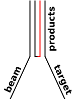
Accelerators are hard to build, and we don’t want to make the accelerator much bigger than it has to be. Therefore, we don’t want to consider all possible versions of equation 26, but only the most energy-efficient versions. The minimum total energy will be achieved in the special case where the products of the reaction have the minimum kinetic energy. That means the products will not be moving relative to each other. This is fairly obvious when you think about it in the center-of-mass frame, as shown in figure 10.
Note that figure 10 is not intended to be quantitatively correct. At this stage of the analysis, we don’t know enough to make a quantitatively correct diagram, but it is a good idea to make some sort of diagram anyway. Very often there is an iterative process:
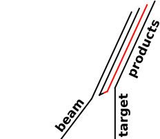
Now let’s switch from the center-of-mass frame to the lab frame. In this frame, we will see the four product particles come flying out the backside of the target in a cluster, as shown in figure 11. In a later step, you can extract the antiproton from the cluster, perhaps by applying magnetic and/or electric fields.
Now that we have a good qualitative picture of what’s going on, we can calculate the required energy. Previously we used the law of conservation of baryon number; now we use conservation of spacetime momentum.
Some reminders: The spacetime momentum is a vector. (See reference 9 for details on what we mean by “vector”.) It is conserved no matter what reference frame (if any!) we choose. If we do choose a frame, we can pick apart the spacetime momentum into components, each of which is separately conserved. The timelike component is the energy, while the spacelike components are the classical 3-dimensional momentum. The spacetime momentum is also called the [energy,momentum] four-vector.
Let pb be the spacetime momentum for the incident beam particle. Similarly pt for the target particle, and pp for the cluster of products.
By conservation of spacetime momentum, we have
| pb + pt = pp (27) |
That is an equation involving spacetime vectors. It is valid in whatever reference frame (if any) you choose. Squaring both sides we get:
| (pb + pt) · (pb + pt) = pp · pp (28) |
We can expand this using the distributive law. That gives us:
| pb2 + pt2 + 2 pb · pt = pp2 (29) |
We know many of the terms in this expression. For starters, we know that
where m is the mass of the incident particle, in accordance with equation 11. (In this section, we have chosen to measure things in units such that c=1.)
The correctness of equation 30a is obvious in the frame comoving with the incident particle. It must then be correct in all frames, since the gorm of any four-vector is invariant.
Similarly, equation 30b is obviously correct in the frame comoving with the target (i.e. the lab frame).
Similarly, equation 30c is obviously correct in the frame comoving with the cluster of products. Don’t forget that the 4 gets squared.
Note the technique used here: We figured out something in one frame, and then expressed it in such a way that it must be true in all frames. This allows us to switch frames. It allows us to carry knowledge from one frame to another. This is a very powerful, very widely-used technique.
Note that this doesn’t happen automatically. You have to engineer the equations so that they have a frame-independent form.
Collecting results, we find
| (31) |
All the equations to this point have been true in all frames. We now specialize to the lab frame. In the lab frame, the target is stationary, so its four-momentum has very simple components:
| pt = [m, 0, 0, 0]@ Lab (32) |
Let’s combine the two previous equations and solve for pb as best we can:
| (33) |
That tells us that in the lab frame, the incident particle must have a total energy of 7m. With a little extra work we could calculate the momentum, i.e. the spacelike components of equation 33 – see below – but we can answer the original design question without that.
Let’s be careful: The design question asks how much energy must be supplied by the accelerator. The incident particle was born with 1m of energy, i.e. its rest energy, in accordance with equation 16 ... so the accelerator only needs to supply 6m of energy, namely the kinetic energy of the incident beam particle.
| EK(required) = 6m (34) |
This is the answer to the design question.
Note: The Berkeley Bevatron was in fact designed to produce antiprotons. The design energy was very nearly equal to what we calculated in equation 34. Actually it was slightly less, because the designers were clever enough to not use a hydrogen target. They used copper. Protons in a non-hydrogenic nucleus are not stationary. Exclusion principle, orbitals, blah-de-blah. If you manage to hit a nucleon that is moving toward the incident beam, its kinetic energy contributes maybe 20% of the reaction energy.
Let’s consider a slightly different scenario. Rather than letting the beam hit a stationary target, we let it collide with another beam moving in the opposite direction. In other words, we arrange that the lab frame is also the center-of-mass frame. This is the situation shown in figure 10.
You should calculate the energy required to produce antimatter using such an apparatus. You will find that the energy per beam is very much less, compared to the scenario considered in section 4.7.
This explains why the Large Hadron Collider (LHC) at CERN is a collider. This has the advantage of much higher energy in the center-of-mass frame, even though it has many drawbacks (compared to using a single beam and let it impinge on a large dense target at rest in the lab frame):
The point remains that the collider geometry allows you to achieve energies that would be simply unobtainable in the stationary-target geometry. The energy advantage is even greater when the reaction products are heavier (not just proton plus antiproton). You can understand this in intuitive terms by looking at figure 11 and invoking the conservation laws: You have to conserve momentum, not just energy. The more momentum there is in the product cluster, the more kinetic energy it has, and then the incident beam has to provide kinetic energy, not just rest energy (i.e. mass). The more energy the beam has, the more momentum it has, which further increases the momentum of the product cluster, magnifying the problem.
Let’s take a closer look at how a ruler (or a log) lines up against various coordinate systems.
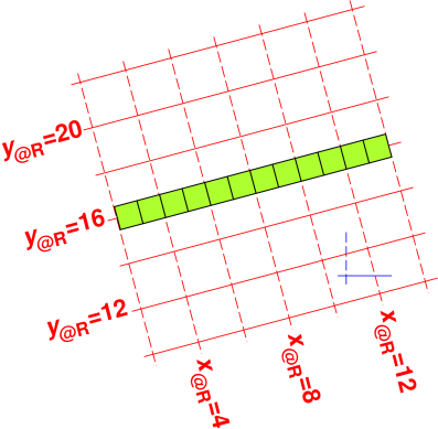
| It should be obvious from figure 12 that the ruler is 12 units long. It extends from x@R = 2 to x@R = 14, and it has no extent at all in the y@R direction (since we are talking about the length, not the width). | It should be obvious from figure 13 that the log is 12 units long. It extends from x@R = 2 to x@R = 14, and it has no extent at all in the t@R direction (since we have taken a snapshot at constant t@R = 12). |
|
| |
| Figure 12: Ruler x|y; Red Coordinate System | Figure 13: Clock x|t; Red Coordinate System | |
|
| |
| Figure 14: Ruler x|y; Blue Coordinate System | Figure 15: Clock x|t; Blue Coordinate System | |
| It should be obvious on physical grounds that the ruler in figure 14 is 12 units long, since it’s the same ruler! Switching to a different coordinate system cannot possibly change the length of the ruler. | It should be obvious on physical grounds that the log in figure 15 is 12 units long, since it’s the same log! Switching to a different coordinate system cannot possibly change the length of the log. The relevant notion of length in this case is the square root of the gorm. |
We can also compute the length
using figure 14, although
this requires slightly more
work. If you look closely at the figure, you can see
that the ruler begins a little to the right of x@B = 2 and
ends a little to the left of x@B = 14, so the x
component is slightly less than 12 units. There is also a nonzero y
component. Specifically, the components are:
|
We can also compute the length
using figure 14, although
this requires slightly more work. If you look closely at the
figure, you can see that the log begins a little to the left of
x@B = 2 and ends a little to the right of x@B =
14, so the x component is slightly greater than 12 units. There is
also a nonzero t component. Specifically, the components are:
|
| When we account for both components we find that the length is indeed 12 units. | When we account for both components we find that the length is indeed 12 units. |
The relevant equation is:
|
The relevant equation is:
|
| The minus sign that shows up in equation 38 is yet another manifestation of the minus sign that we first saw in equation 4. |
| When measuring the length of some object that is oriented at an arbitrary angle in the xy plane, you can’t just measure the x-component and call it quits. You have to account for the x and y components, both. The x@B component is not the length. | When measuring the length of some object that is moving at an arbitrary rapidity in the x direction, you can’t just measure the x-component and call it quits. You have to account for the x and t components, both. The x@B component is not the length. |
This is a basic fact about the geometry of spacetime. We have already seen this in the context of momentum vectors. We used it to calculate the kinetic energy in section 4.3. The only thing that is new in this section is that we have emphasized the pictorial representation (not just the equations) and applied it to position vectors (not just momentum vectors).
| A rotation in the xy plane guarantees that the x-component is less than or equal to the proper length. This has been understood in connection with perspective in painted artwork for many centuries. Artists call it foreshortening. | A rotation in the tx plane guarantees that the x component is greater than or equal to the proper length. Remember that the geometry in timelike directions is non-Euclidean. This could be called forelengthening ... but I’m not sure that term will ever catch on very widely. |
For fast-moving objects, you really need to pay attention to Big Idea #2 if you want to get the right answers. Everybody learned in grade school that x, y, and z are “the” components, and everybody habitually takes them into account when calculating the length. Special relativity tells us that t is also a component, and must be taken into account when calculating the length.
Let’s turn our attenion 90 degrees, and see what happens if we want to calculate elapsed time (rather than length). If you have accepted Big Idea #2, the results will be completely routine ... but if you have not yet fully accepted the idea that spacetime is four-dimensional, you are in for a surprise.
The following figures are the same as the preceding figures, except that we consider an object that extends in some non-x direction.
|
| |
| Figure 16: Ruler y|x; Red Coordinate System | Figure 17: Clock t|x; Red Coordinate System | |
|
| |
| Figure 18: Ruler y|x; Blue Coordinate System | Figure 19: Clock t|x; Blue Coordinate System | |
| The ruler in figure 16 and figure 18 is 12 units long. It’s the same ruler! | The elapsed time in figure 17 and figure 19 is 12 units. It’s the same clock! The start-event is the same in both figures. The end-event is the same in both figures. For an explanation of what we mean by the special term event, see reference 10. |
| You can see in figure 18 that the y@B component is slightly less than 12. | You can see in figure 19 that the t@B component is slightly greater than 12. |
The relevant equation is:
|
The relevant equation is:
|
Again: For fast-moving objects, you really need to pay attention to Big Idea #2 if you want to get the right answers.
| When you measure the x component, it’s usually obvious that there are other components you need to worry about. | When you measure the t component, if you don’t understand special relativity, it won’t be the least bit obvious that there are other components you need to worry about. |
| You have to account for all the components. The y@B component is not the proper length. | You have to account for all the components. The t@B component is not the proper time. |
Whenever a calculation produces a result that is simpler than expected, it is a good practice to see if there is a simpler way of obtaining the same result.
The result obtained in section 4.7 falls into this category. It was not obvious a priori that the answer would be a round number, so we have to suspect there is a more elegant way to obtain this number, and a better way of understanding where it comes from. Indeed there is. With the aid of the spacetime diagrams, you can solve the whole problem in your head, using no mathematics beyond addition, subtraction, multiplication and division ... plus a qualitative notion of rotation in the xt plane. (This is even simpler than the method presented in section 4.7, which uses vectors and dot products.)
This method is easier and more elegant, but it is less powerful in the sense that it depends on the symmetry of the situation. In contrast, the spacetime vector method would work even in less-symmetrical situations.
In the center-of-mass frame, as we can see in figure 20, the product particles have no kinetic energy, so their total energy is just their rest energy, for a total of 4m. By conservation of energy, that means the incident particle and the target particle have 4m of energy total, or 2m apiece. That means that for each of them, the energy is evenly split: 1m of rest energy and 1m of kinetic energy.
Similarly, we can create a spacetime diagram of the situation in the lab frame, simply by boosting the worldlines in figure 20, thereby producing figure 21. It takes only a few moments to do this using the transform dialog in the drawing program, as discussed in section 7.3.
It is no accident that the angle θ1 in figure 20 is the same as the angle θ1 in figure 21. The two figures show the same physics, and differ only by a rotation of the reference frame. The rotation that reduces the velocity of the target from θ1 to zero increases the velocity of the product cluster from zero to θ1. This fact – combined with the fact that θ1 corresponds to an even split – tells us that the product particles’ energy in the lab frame is also evenly split: Each particle has 1m of rest energy and 1m of kinetic energy. The total energy for the four-particle cluster is 8m.
We have used the idea that each particle’s energy is determined by its mass and its rapidity, and the rapidity θ1 is the same in both figures.
The target particle and the incident particle are each born with 1m of rest energy, so the accelerator must supply 6m of additional energy, to reach the required total of 8m.
This is the answer to the question: The accelerator must impart 6m of kinetic energy to the incident particle. In engineering units, the mass of a proton is about a GeV (.938 GeV) so we must design the accelerator to produce about 6GeV.
We have solved the problem without worrying too much about the numerical value of θ, but we can quantify it if we wish, as follows: The short version is that the energy varies in proportion to cosh(θ).
The long version of the same story goes like this: The spacetime momentum of any particle in its own rest frame has components [m, 0, 0, 0] in accordance with equation 23. In any other reference frame, the spacetime momentum has components [m cosh(θ), m sinh(θ), 0, 0] as you can see by applying equation 49.
That tells us that in figure 20 and figure 21, the rapidity is θ1 = arccosh(2). We know that arccosh(2) = 1.31696, but we didn’t really need to know that to solve the problem.
The figures in this section (figure 20 and figure 21) are drawn with the quantitatively-correct angle, θ1 = 1.31696. This is in contrast to section 4.7, where the sketches (figure 10 and figure 11) used the artistically-licentious value of θ1=0.5. It turns out that the diagrams with the quantitatively-correct angles don’t tell us much beyond what the non-quantitative sketches told us. In some ways the sketches are actually easier to interpret.
Sometimes you want a quantitatively correct blueprint, and sometimes you would rather have a sketch where some features have been exaggerated for clarity. When in doubt, make one of each. Keep in mind that the diagram will not usually do the whole calculation for you; instead you should expect the diagram to guide the calculation. Then the calculation can guide the construction of a better diagram, and so on, iteratively.
Remark: If we turn our attention to the incident beam particle, and examine its energy-versus-rapidity relationship in the two coordinate systems, we discover that we have just proved that arccosh(7) = 2 arccosh(2). This can be understood as a special case of a trigonmetric identity, namely the double-angle formula cosh(2θ) = 2cosh2(θ)−1.
How far can a fast-moving muon travel before it decays? The answer, as measured in the obvious way, is a lot longer than the muon lifetime multiplied by the speed of light.
Muons are subatomic particles. You can obtain a few of them quite cheaply, since they are produced all the time by cosmic rays striking the upper atmosphere. (They are also produced by particle accelerators ... but those are not so widely available.)
It is known from a combination of theory and experiment that muons decay with a half-life of 1.56 microseconds. That’s the proper time, measured in the frame of the muon itself. However, the available muons are not stationary in the lab frame. Let’s consider the case where they have a rapidity (relative to the lab frame) of θ = 3 radians, which means their classical velocity (i.e. reduced velocity) is v = dx/dt = tanh(3) = 99.5% of the speed of light.
Let’s calculate how far they will travel. A “rate × time” calculation naïvely using the muon’s proper time would suggest that half of them will survive for 1,560 feet ... but that is not the right answer in the lab frame. It’s off by a factor of 10.
Here is the correct calculation: We know the lifetime in terms of proper time, τ½= 1.56µs. When the muon is not at rest with respect to the lab, the t@lab component is not the proper time. That is, the time you measure with a stopwatch in the lab frame is not the muon’s proper time. (It is the stopwatch’s proper time, but that’s the answer to the wrong question.)
Spacetime geometry tells us that the t@lab component will be longer than τ by a factor of dt/dτ = cosh(θ) = cosh(3) = 10.
As another way of saying the same thing, the spacetime velocity of the muon is:
| (41) |
Let’s be clear:
| (42) |
| (43) |
It is nice that the explanation is independent of the internal details of the muon. This independence keeps things simple. More importantly, it increases our confidence in the principle of relativity. It guarantees that you can measure proper time using any method you choose: muon clocks, photon clocks, cuckoo clocks, biological aging processes, and/or whatever else you can think of. In every case, proper time gets projected onto the lab frame in the same way, because the projection has got nothing to do with how the clocks work; it is entirely explained by the geometry and trigonometry of spacetime.
To say the same thing the other way: Suppose the dt/dτ did depend on the internal workings of the clock.
The following diagrams may make the situation easier to visualize. Recall that most of the previous spacetime diagrams considered the situation where the rotation angle was 0.25 radians. Figure 22 shows the situation where the rotation angle (i.e. the rapidity) is a full radian. You can see that the red reference frame is rather seriously stretched in one direction and squashed in another direction. If we increase the angle to 2 radians, as in figure 23, things are so badly stretched and squashed that the diagram is hard to interpret. Three radians would be so bad that it’s not worth showing the diagram, even though that is the case that corresponds to our muon example. At some point you have to trust the equations ... and/or use your mind’s eye to extrapolate on the basis of figure 22 and figure 23.
In spacetime there is a nonlinear relationship between slopes and angles. It is closely analogous to the situation in ordinary Euclidean space; almost but not quite identical.
| Figure 24 shows part of a circle, in green. This is what we get if we consider an ensemble of vectors, rotated in the xy plane by various amounts. The small black circles represent angles from 0 to 1 radian, in steps of 1/4 radian. | Figure 25 shows part of a hyperbola, in green. This is what we get if we consider an ensemble of vectors, rotated in the xt plane by various amounts. The small black circles represent angles from 0 to 1 radian, in steps of 1/4 radian. |
|
| |
| Figure 24: Rotations in the xy Plane | Figure 25: Rotations in the xt Plane | |
The points in figure 24 satisfy
equation 44, which in some sense defines what we mean by
circle:
|
The points in figure 25 satisfy
equation 45, which in some sense defines what we mean by
hyperbola:
|
| I did not, however, plot figure 24 by solving the equation x2 + y2 = 1. Instead I plotted x=cos(θ) and y=sin(θ) for various values of θ. | I did not, however, plot figure 24 by solving the equation t2 − x2 = 1. Instead I plotted t=cosh(θ) and x=sinh(θ) for various values of θ. |
| The functions sin(), cos(), tan(), etc. are called circular trig functions. | The functions sinh(), cosh(), tanh(), etc. are called hyperbolic trig functions. |
| The trigonometric identity cos2 + sin2 = 1 guarantees that the dot product between any two vectors is invariant under rotations in the xy plane. | The trigonometric identity cosh2 − sinh2 = 1 guarantees that the dot product between any two vectors is invariant under rotations in the tx plane. |
The minus sign that shows up in equation 45 is essentially the same as the minus sign that shows up in equation 4. It is the hallmark of non-Euclidean geometry.
Note that figure 25 conveys essentially the same information as figure 6. The main difference is that each is transposed relative to the other. That is, we plot t horizontally and x vertically in one figure, and vice versa in the other.
The choice of which variable to plot in which direction is a matter of taste. In figure 6 and figure 25 it looks better to plot the timelike variable (energy) vertically. Indeed there is a tradition in the relativity business, dating back to Minkowski, of plotting the timelike variable vertically. (This conflicts with the high-school physics tradition of plotting time horizontally.)
No matter what the tradition, we are allowed to make exceptions. Let’s plot time horizontally, to facilitate comparison with figure 3 and figure 5. This will help explain the idea of slope in spacetime.
Let’s revisit the idea of slope. Figure 26 shows a ruler sitting in ordinary Euclidean space, while figure 5 shows a clock moving through spacetime.
|
|
| |
| Figure 26: Ruler Plus Blue Coordinate System | Figure 27: Clock Plus Blue Coordinate System | |
In figure 26, for small rotation
angles, the slope is proportional to the angle θ. For larger
angles, the relationship is nonlinear: the slope is given
by:
|
In figure 5, for
small rotation angles, the reduced velocity is proportional to the angle
θ. For larger angles, the relationship is nonlinear:
the reduced velocity is given by
|
The rotation matrix for a rotation in the
xy plane is:
This uses circular trig functions ... and one of the matrix elements has an important minus sign. |
The rotation matrix for a rotation in the
tx plane is:
This uses hyperbolic trig functions ... and there are no minus signs. |
Here is equation 49 again, with more context, to
provide a hint about what the matrix elements mean:
|
Summary: If you’ve been paying any attention at all, you will have noticed that spacetime is not quite the same as ordinary Euclidean space, but there are profound similarities:
| (51) |
We continue this line of thought in the next section.
The results of section 4.3 have a simple, powerful, and elegant interpretation in terms of rotations. This was foreshadowed in section 4.4.
| Refer to figure 24. Suppose we start out with a vector of length m, pointing in the y-direction. If we rotate it by a small angle θ, to first order the y-component is unchanged. To second order, the y-component decreases by ½mθ2. This comes directly from the Taylor expansion of the cosine function. If you don’t believe me, you can use a calculator to evaluate cos(θ) for θ = 0.01 radians, 0.02 radians, et cetera. | Refer to figure 25. Suppose we start out with a vector of length m, pointing in the t-direction. This represents the rest-energy of the particle. When the particle is “at rest” in the conventional three-dimensional sense, really it is moving in the t direction at a rate of 60 minutes per hour. If we rotate it by a small angle θ, to first order the t-component is unchanged. To second order, the t-component increases by ½mθ2. This comes directly from the Taylor expansion of the hyperbolic cosine function. If you don’t believe me, you can use a calculator to evaluate cosh(θ) for θ = 0.01 radians, 0.02 radians, et cetera. |
| For small angles, θ is equal to the 3-velocity (accurate to second order). Therefore the increase in energy is equal to ½mv2. This is the difference in energy between a particle with 3-velocity v and a particle at rest ... in other words, the kinetic energy. Special relativity predicts that the kinetic energy is ½mv2 in the classical limit, which is the correct classical result (for a particle of nonzero mass). |
| Classically we do not observe the rest energy. We only observe changes in energy. In relativity, having a rest energy equal to mc2 is the only value of rest energy that is consistent with the classical kinetic energy in the correspondence limit, and consistent with the idea that a boost is a rotation in the xt plane. |
Let’s take another look at the red coordinate systems in figure 12 and figure 13.
The first thing we notice is that each of them is tilted relative to the corresponding blue coordinate system. (There is a vestige of the blue coordinate system in the middle of each diagram, to facilitate this comparison.) However, there are two different types of tilt:
| In figure 12, both the contours of constant y and the contours of constant x are tilted counterclockwise (relative to the blue system). The whole system looks like it has been rotated. | In figure 13, the contours of constant x are tilted counterclockwise, while the contours of constant t are tilted clockwise. Superficially, the whole system looks like it has been skewed ... but really it is has just been rotated in the tx plane. |
| This is characteristic of conventional circular trigonometry. | This is characteristic of hyperbolic trigonometry. This is yet another manifestation of the minus sign that we saw in equation 4. We have seen the same minus sign again and again. |
| In figure 12, the contours of constant x are orthogonal to the contours of constant y ... as is apparent from the diagram. | In figure 13, the contours of constant t are orthogonal to the contours of constant x ... even though this is not readily apparent from the diagram. |
Here’s the deal: In figure 13, the lines on paper are merely symbols that represent the actual contours in spacetime. The lines on paper are obviously not orthogonal ... but the contours that they represent are orthogonal.
| |
Let’s be clear: The diagram-on-paper is not an entirely faithful representation of what’s going on in spacetime. The paper has two spacelike dimensions, but we’re trying to use it to represent a situation that has one spacelike and one timelike dimension. The contours are orthogonal (if you think about what’s happening in spacetime) but they don’t look orthogonal (if you only think about what’s happening on the paper).
Let’s do an example. Let’s consider two basis vectors in the red frame:
| (52) |
It should be obvious that these two vectors are orthogonal. If it’s not immediately obvious, you can check it using equation 4 and especially equation 6.
Meanwhile, the same two vectors can be analyzed in the blue frame:
| (53) |
If we take the dot product between these two vectors, using the blue-frame expansion on the LHS of equation 53, we find it is equal to −cosh(θ)sinh(θ) + sinh(θ)cosh(θ), which is always zero, confirming that the vectors are orthogonal.
One way to explain this is to say that the minus sign that is present in the dot-product rule (equation 4) makes up for the minus sign that is missing from the rotation matrix (equation 49).
This is one of the few truly tricky things about special relativity: Whereas a diagram such as figure 12 is a remarkably faithful representation of the actual rotated contours, a diagram such as figure 13 is not an entirely faithful representation. You need some skill to interpret it correctly.
In any case, the fact remains that spacetime diagrams are your friend. Having a spacetime diagram is always better than not having one. The main points of a spacetime diagram are easy to interpret. It takes some skill to interpret the fine points, but this is a skill that can be learned.
Let’s impose two coordinate systems (red and blue) on the same physics. Specifically, let’s start with figure 9 and superimpose the corresponding red coordinate system. The result is shown in figure 28.
The black line in figure 28 represents the worldline of a fast-moving particle. It has a reduced velocity v = [c, 0, 0]. Remarkably, its reduced velocity is the same in either frame (and in any other rotated frame, for any rotation in the tx plane).
The other diagonal (not shown) has the same property: A particle with reduced velocity v = [−c, 0, 0] has the same reduced velocity in any frame. No other directions in the tx plane have this property.
This is very unlike ordinary spacelike rotations, where no vector in the plane of rotation is unaffected by rotations.
When you calculate the reduced velocity in the two different frames, the Δt and the Δx will be different. You can see by looking at the starting-point and ending-point of the black line, and evaluating the coordinates of these points in the two different frames. However, the ratio Δx/Δt will be the same in both cases.
If you take an ordinary particle (such as an electron) and boost it to higher and higher rapidity, its world line gets closer and closer to the black line in figure 28. So, loosely speaking, the black line corresponds to a world line where the x-component of the spacetime velocity is infinite.
For a massless particle (such as a photon) moving in the x direction, its worldline coincides with the black line. The spacetime velocity of such a particle is undefined.
Interestingly enough, the spacetime momentum is perfectly well defined for massless particles, even though the spacetime velocity is not. Obviously you cannot compute the spacetime velocity from the spacetime momentum via the formula u=p/m, since the mass is zero. Still, you can measure the energy and the momentum directly.
For a massless particle, E2 always equals pxyz2, no matter what frame (if any) you choose, in accordance with equation 13.
Important tangential remark: The speed “c” is conventionally called the speed of light. However, the phenomenon we are describing here is absolutely not restricted to light. The speed we are talking about throughout this document is a geometrical property of spacetime. Rather than calling it the speed of light, you could call it the speed of diagonals in spacetime.
| |
For details on this, see reference 11.
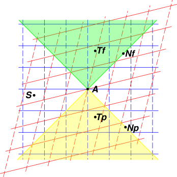
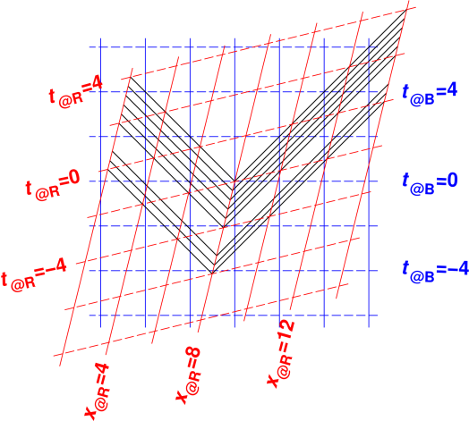
In figure 29, let’s take point A to be our reference point. The green-shaded region is interior of the future light cone of point A, and the yellow-shaded region is the interior of the past light cone of point A.
The surface of each light cone consists of paths corresponding to the speed of light, hence the name. The light cone is independent of the choice of reference frame. This is guaranteed by the invariance of the speed of light. You can see in the diagram that the light cone (i.e. the edge of the shaded region) has a slope dx/dt = 1 in both the red frame and the blue frame. The same is true for any other reference frame.
There are six frame-independent things we can say about the various points in the diagram:
Those six itemized statements are frame-independent. In contrast, it is not possible to decide, in any invariant way, whether point S occurs before or after point A. It is earlier than A in the blue reference frame, but later than A in the red reference frame, as you can see by following the contours of constant t in each frame. This is generally referred to as the breakdown of simultaneity at a distance but it’s even worse than that; it’s the breakdown of time-ordering at a distance.
To summarize: Any given point has a past light cone and a future light cone. We can arrange events “in chronological order” if they are separated by timelike or lightlike intervals ... but not if they are separated by spacelike intervals.
In this section, we analyze the addition of velocities in 1+1 dimensions, i.e. one timelike dimension plus one spatial dimension. (The case of multiple spatial dimensions is discussed in section 4.18.) For massless waves (aka particles) the primary effect is a change in frequency, called the Doppler effect. For things with nonzero mass, there is also a change in velocity.
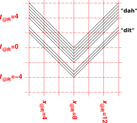
Suppose we use a signal lamp to send Morse code letter “A” (dit-dah). Our signal lamp is similar to the one shown in figure 30, except that it sends light in both the +x and −x directions.
As usual, the first step is to draw some spacetime diagrams. In the frame of the transmitter, the relevant diagram is shown in figure 31. We choose coordinates such that the transmission ends t@R=0.
The black lines represent the world-lines of the photons. As another useful way of interpreting the same diagram, the spacing between adjacent black lines represents one cycle of the electromagnetic wave.
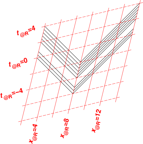
We now consider what things look like in the frame of a receiver. The transmitting ship is moving in the +x direction relative to the receiver.
The situation is shown in figure 32. A less-cluttered version is shown in figure 33. Note that I drew figure 31 freehand, and then computed figure 32 by applying a transformation matrix (as in equation 64). This guarantees that all the relationships are correct. The angle of the boost is θ = 0.25 radian.
|
| |
| Figure 32: Light Pulses in the Frame of the Blue Receiver | Figure 33: Light Pulses in the Frame of the Blue Receiver Only | |
| Consider a receiver who is at rest in the blue reference frame, and is positioned astern of the transmitter, i.e. at a lesser x-coordinate. This corresponds to the upper-left corner of figure 32 and figure 33. The light is red-shifted. You can see that in the diagram, because there are fewer cycles per unit t@B; specifically, the same number of cycles is packed into a larger amount of t@B. | Consider a receiver who is at rest in the blue reference frame, and is positioned ahead of the transmitter, i.e. at a larger x-coordinate. This corresponds to the upper-right corner of figure 32 and figure 33. The light is blue-shifted. You can see that in the diagram, because there are more cycles per unit t@B; specifically, the same number of cycles is packed into a smaller amount of t@B. |
Last but not least, consider a receiver who is in another ship, comoving with the transmitting ship. This receiver sees no Doppler shift whatsoever. This is obvious if we analyze the situation in the red frame, as in figure 31. It is less obvious, but no less true, if we analyze the situation in the blue frame, as in figure 34. Comparing the upper-left and upper-right corners of the diagram, we see the same number of cycles per unit t@R.
Note that you have to be rather careful about how you measure t@R. This is discussed in more detail in section 7.2.
For some discussion of misconceptions that can arise when analyzing this sort of situation, see reference 11.
In this section, we analyze the addition of velocities in 1+2 dimensions, i.e. one timelike dimension plus two spatial dimensions. (The case of a single spatial dimensions is discussed in section 4.17.) That is to say, relative to the red frame, a wave (or particle) is moving in one direction, and the blue frame is moving in some other direction. We want to know what this looks like in the blue frame. The effect on the frequency of the wave is called the Doppler effect. The effect on the direction of propagaion of the wave is called aberration.
We start by reviewing the familiar low-speed situation. The main purpose here is to establish the interpretation of the diagrams.
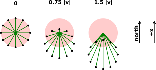
So ... Suppose we are having a slug race. We take 12 slugs and start them all at the same location. They immediately begin slithering away from each other in 12 different directions, all at the same speed |v|. The situation relative to the red reference frame is shown in the diagram on the left in figure 35. The green lines represent velocity vectors. Position is not represented in these diagrams, and is not relevant, since we are considering the initial situation, when all 12 slugs are at the same location.
Now let’s look at the same situation in the blue reference frame, which is moving northward (relative to the red reference) frame at a rate equal to three quarters of the slug-speed |v|. This situation is shown in the middle diagram in figure 35. In this frame, the slugs that were moving northward now have a smaller speed (as seen near the 12:00 position in the diagram), while slugs that were moving southward have a greater speed (as seen near 6:00).
Continuing that line of thought, let’s look at the same situation in a frame that is moving northward even faster, at a speed 1.5 times the slug-speed |v|. Even the slugs that were moving northward in the red frame are moving southward in this frame.
There is nothing tricky going on here. These results should be familiar. They are well explained by classical physics. Of course special relativity agrees with classical physics in the low-speed regime.
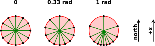
Let’s do the same experiment again, except using photons instead of slugs. Photons are quite a bit faster than slugs.
That is, we set off a flash of light. Twelve photons fly outward, in 12 different directions, all with the same speed |v| = c. The situation as seen in the red reference frame is shown in the left diagram in figure 36.
Now let’s look at the same situation in the blue reference frame, which is moving northward (relative to the red frame) with a rapidity of 1/3rd of a radian. (That’s about 32% of the speed of light.) This is shown in the middle diagram in figure 36.
Continuing that line of thought, let’s look at the same situation in a frame that is moving northward with a rapidity of 1 radian. (That’s about 76% of the speed of light.) This is shown in the right diagram in figure 36.
You can see that in all cases, in all frames, the photons travel with speed |v| = c.
Note that no matter how fast your frame is moving northward, it will never catch up with the northward-moving photon.
Here’s how to calculate such things. The executive summary is very simple and easy to understand: Promote the classical velocity from a 3-vector to a spacetime vector, boost the spacetime vector, and then convert it back to a 3-vector.
Here are the details. We assume the initial photon direction is known. Since the speed |v| is known to be c, we know the entire classical velocity vector v.
| (54) |
You should take a moment to verify that the gorm of q is zero, as it should be for a massless particle such as a photon.
If we know the energy E of the photon, we can multiply both sides of equation 54 by E/c2 to obtain the spacetime momentum. The photon doesn’t have any mass, but E/c2 has dimensions of mass, so this passes the dimensional-analysis check.
| (55) |
If we don’t know the energy, or don’t care, we can set E/c2=1 and forge ahead. It doesn’t matter, because the whole calculation is linear, and E is effectively just a scale factor.
As a further check, note that if we calculate v from p, by plugging equation 55 into equation 82e, we get back the v we started with.
| (56) |
Beware that the boost angle (aka rapidity) θ will be negative in our example, since the red frame is moving in the −x direction relative to the blue frame.
This 3-step procedure can easily be reduced to a single-step closed-form expression, but the resulting expression is much harder to remember, and not any easier to use in practice.
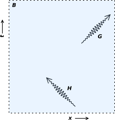
Let’s do an example. Suppose we have a source (perhaps positronium) that is moving relative to the lab frame at some rapidity ρ in the x direction. Then the source decays into two photons. Suppose that by good fortune the photons are moving in the x-direction. In the center-of-mass frame, we know by symmetry that the two photons have the same frequency, which we can call q. In the lab frame, they will be Doppler shifted.
We name the photons G and H, and use the following notation for the photon properties:
| (57) |
The notation can be read from right to left; for example B∘p∘1 can be read as the x-component of the momentum of photon B. This notation is analogous to the “dot qualifier” notation used to specify class membership in object-oriented programming languages such as C++. (If the previous sentence didn’t mean anything to you, don’t worry about it.) This notation gives us a systematic way to specify everything that needs to be specified. This stands in contrast to subscripts, which are often used in unsystematic ways. For example, pA uses a subscript to denote that momentum of A, while px uses a seemingly-equivalent subscript to denote the x-component of the momentum.
Using this notation, the momenta in the center-of-mass frame can be written as:
| (58) |
Applying the transformation equation 56, we find the Doppler-shifted momenta in the lab frame:
| (59) |
The photon frequency is proportional to its energy, in accordance with the famous equation E = ℏω. Equation 58 tells us that when one photon is upshifted by a certain factor, the other photon is downshifted by the same factor. Therefore the product of their frequencies is invariant, as we see in equation 60a.
|
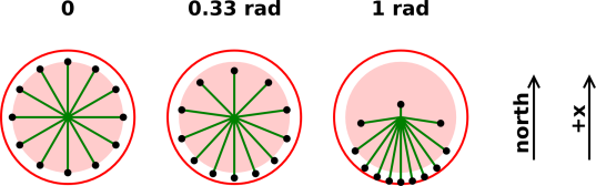
Now let’s consider a particle that is neither super-slow (slug) nor super-fast (photon). That is, the particle has some nonzero mass, but it is moving fast enough that the classical approximations do not apply. The situation is shown in figure 37. Here (as in other figures in this section), the red ring represents the speed of light. The pink disk serves as a reminder of what the velocity vectors were doing originally, when the blue frame was not moving relative to the red frame.
In all cases, we use the same 3-step procedure: Figure out the particle’s spacetime momentum, boost the spacetime momentum, and then (if necessary) convert that to a classical velocity. All the figures in this section are computed using the same code, just using different parameters. The parameters are given in the following table:
| | m | | |pxyz| | | |v| | |
| figure 35 | | 1 | | 0.01 | | 0.01 |
| figure 37 | | 1 | | 1.5 | | 0.832 |
| figure 36 and figure 38 | | 0 | | 1.5 | | 1 |
You can see that in terms of the speed of the spreading particles, figure 37 is intermediate between figure 35 and figure 36. This demonstrates yet again the power and elegance of special relativity: It provides us a unified understanding of the low-speed limit, the high-speed limit, and everything in between.
It must be emphasized that this approach is quite general. It treats massive particles and massless particles the same way. We have not made use of any detailed knowledge of the electromagnetic field, even during the discussion of photons in section 4.18.2; we merely assumed that the photon was a particle with some energy and momentum but no mass.
One famous application has to do with the so-called “aberration of starlight” which was first noticed experimentally hundreds of years ago. The earth in its orbit is moving at about 0.01% of the speed of light, and the direction changes every 6 months. This has a noticeable effect on the apparent direction from which light arrives from distant stars; that is, the stars appear to shift position.
For some purposes, 0.01% is a sufficiently small number that a first-order semi-classical approximation is satisfactory, and you don’t need to understand special relativity to calculate the aberration. On the other hand:
We also care about the Doppler part of the equation (not just the angular aberration). There are bench-top atom-trapping experiments where the frequencies are so finely tuned that the fully-relativistic Doppler formula is needed. There are also innumerable applications in elementary particle physics.
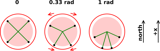
Note that the transformation matrix equation 56 leaves unchanged the two components of the spacetime velocity that are transverse to the boost, i.e. transverse to the relative velocity between the two frames. This is simple, and makes perfect sense in four dimensions. It agrees with your intuition at low speeds, where the classical velocity and the spacetime velocity behave pretty much the same. You can see that each dot in figure 35 moves straight down the page as the velocity of the blue frame (relative to the red frame) increases.
This stands in contrast to the situation at higher speeds, where the transverse components of the classical velocity do change. You can see in figure 38 that the upper two dots initially move away from the midline, while the lower two dots move toward the midline.
The only reason for mentioning it is to warn you that it is not worth thinking very much about this phenomenon in three dimensions or in terms of the classical velocity. Far and away the simplest way to explain what is going on is the three-step procedure given above: promote the 3-vector to a spacetime vector, boost the spacetime vector, and then convert back to a 3-vector.
For a massive particle, we can understand this as follows: The boost does not affect the transverse components of the spacetime velocity (u = d(position)/dτ), but it does affect the transverse components of the classical velocity (v = d(position)/dt). That’s because it affects dt. Remember that dt/dτ = cosh(θ) = γ.
For a massless particle such as a photon, you can make almost the same argument, but you have to phrase it in terms of the spacetime momentum rather than the spacetime velocity. (A massless particle doesn’t have any proper time, and its spacetime velocity components are either undefined or infinite ... but its spacetime momentum is still perfectly well behaved.)
| In any case, the point is that the physics is simple in four dimensions. | Describing the same physics in classical terms is sometimes not so simple. |
| In particular, a boost leaves the transverse components of the four-velocity unchanged, which is nice and intuitive. It is conceptually simple and in every other way simple. | The classical description of the transverse components is tricky. By far the biggest source of confusion is the fact that the 3-velocity v is the reduced velocity. It is not simply the spatial part of the spacetime velocity! It is reduced by a factor of γ. This messes with the transverse components of v. |
| |
This is quite different from most other things (including position and momentum), where the classical vector is just the spacelike part of the spacetime vector.
Consider the following puzzle:
Suppose a spacecraft starts from rest and accelerates in a straight line such that the passengers feel one Gee for one year. How fast are they going at the end of the year?
This puzzle is quite easy to solve, if you think about it the right way. The central idea here is the same as in section 4.2.
We further assume that “how fast” refers to the classical speed (|v| = |dx/dt|) in the lab frame. Unfortunately, when non-experts speak of “the” velocity they usually mean the classical velocity, i.e. the reduced velocity. In contrast, anybody who is interested in the spacetime velocity (u = dx/dτ) is probably clever enough to ask for it by name, explicitly, i.e. spacetime velocity.
Therefore the answer will depend on v = tanh(θ), and all we need to do is find the value of the rapidity, θ.
We assume that “one year” means one year of proper time, since that is what the passengers experience. (The projection of this time onto the lab frame will cover more than one year of lab-time.)
It may seem a bit inconsistent to use lab-frame velocity and spacecraft-frame proper time. However, we can express everything in a common frame as follows: After one year of proper time, the passengers look out the window. How fast is the original lab frame receding, relative to the spacecraft?
Rotations have the nice property that if you rotate by an angle θ1 and then rotate by an additional angle θ2, the combined effect is the same as a single rotation by an angle (θ1 + θ2). That is, for compound rotations, the angles are additive.
Therefore we introduce the idea of an instantaneously comoving reference frame. An example shown in red in figure 39. In this frame, the ship has a small velocity and is undergoing a gentle acceleration, so we can use classical physics to understand what is happening in this frame. (For details on this, see section 4.20).
Elapsed time in this frame is equal to the ship’s proper elapsed time, for any interval of time that is not too large. We conclude that the whole flight is described by saying that the rapidity is proportional to proper time. The constant of proportionality is 32.7 microradians per second. That’s the acceleration, in spacetime units.
It is a remarkable coincidence that earth’s surface gravity times the earth’s year is very nearly equal to 1 radian.
The small black circles in figure 39 correspond to rapidities from 0 to 1 radian in steps of 0.25.
Remarks: This is obviously a made-up puzzle, not a real-world application, but it is easy and fun, and illustrates some useful principles. Also, there are some real-world problems that are not too different from this, for instance having to do with particle accelerators.
The idea of using a succession of instantaneously-comoving unaccelerated reference frames is very powerful. In each such frame, the physics is simple. You just have to find a way to add up the contributions from all such frames.
We have already answered the question that was posed in section 4.19, but the method of solution has some interesting features that we can explore.
The instantaneously comoving reference frame in figure 39 is an unaccelerated reference frame. (You could use an accelerated frame, but that would be unnecessary extra work.) We emphasize that this frame is not attached to the spaceship. It is just something that happens to be in the neighborhood as the spaceship passes by.
Indeed, it does not even need to be exactly comoving; all we really need to do is choose a frame where the ship is moving slowly (relative to the chosen frame) ... sufficiently slowly that we can confidently apply the classical (non-relativistic) laws of physics.
Whenever you encounter a new idea, it is smart to turn it over in your mind, checking whether it is consistent with other things you know, and seeing how it fits in. It is smart to be skeptical.
The technique of using an instantaneously comoving reference frame fits in as follows: It is quite a direct application of the basic principle of relativity, as set forth in section 3.1: The spaceship does not care about the distant past or the distant future. It does not care how things look in any particular reference frame. In figure 39, we are free to ignore the blue coordinate system and use the red reference system. At times when the ship’s rapidity is approximately 0.5 radian, the ship is moving only slowly with respect to the red reference frame, and the situation is entirely classical. Assuming the ship is in empty space, unaffected by outside influences, there is no experiment anyone can do to demonstrate that the ship is moving relative to the blue reference system.
The skeptical reader may also be wondering about the assertion that for a compound rotation, the angles are additive. For a rotation in the tx plane, we know that the velocities are not additive. We know that any nonlinear function of the angle (such as angle cubed) is not additive. So what is special about the angle that makes it additive? Here are three answers:
The whole flight is described by the equation:
| (61) |
which we can immediately integrate to find that θ(τ) = (a/c)τ.
Therefore the spacetime velocity is
| (62) |
which is consistent with saying the classical velocity is tanh(aτ), as we did in section 4.19.
We can immediately integrate equation 62 to find the position:
| (63) |
This tells us that the ship’s worldline (shown in dark green in figure 39) is a hyperbola. Indeed, steadily accelerated motion is sometimes referred to as hyperbolic motion in spacetime.
For yet more discussion of acceleration in spacetime, including sideways acceleration and circular motion, see reference 12. For situations involving large objects and/or large accelerations, see reference 13.
Recall that figure 12 and figure 14 show a ruler that extends mostly in the x-direction in the two coordinate systems we have been considering. We now look at those figures again. In each case, we pair it with the analogous situation in the tx plane.
|
|
| |
| Figure 40: Ruler x|y; Red Coordinate System | Figure 41: Clock x|t; Red Coordinate System | |
|
|
| |
| Figure 42: Ruler x|y; Blue Coordinate System | Figure 43: Clock x|t; Blue Coordinate System | |
We contrast that with rulers and logs that extend mostly in the other (non-x) direction.
|
|
| |
| Figure 44: Ruler y|x; Red Coordinate System | Figure 45: Clock t|x; Red Coordinate System | |
|
|
| |
| Figure 46: Ruler y|x; Blue Coordinate System | Figure 47: Clock t|x; Blue Coordinate System | |
Note the contrast:
The breakdown of simultaneity at a distance is something we learn by taking seriously the idea that time is the fourth dimension, and taking seriously the correspondence between rotations in the xy plane and rotations in the tx plane. Let’s be clear: To first order, every small1 rotation does two things:
| For a small rotation in the xy plane, a vector that extends in the x-direction picks up a small y-component ... and ... a vector that extends in the y-direction picks up a small negative x-component. | For a small rotation in the xt plane, a vector that extends in the t-direction picks up a small x-component (which corresponds to the ordinary classical velocity) ... and ... a vector that extends in the x-direction picks up a small t-component (which corresponds to the breakdown in simultaneity at a distance). |
In principle, it is straightforward to observe this breakdown. We can observe the time that the left clock strikes zero. This is an event in spacetime, i.e. something that happens at a specific time and place; for details on what we mean by this, see reference 10. Similarly we can observe the time that the right clock strikes zero. This is another event. These are not simultaneous events according to the blue contours of constant time.
So another way of making the same point is to say that to first order, a small difference in velocity – i.e. a small rotation in the xt plane – has two consequences:
We can understand these two things mathematically by looking at the rotation matrix, equation 49, which we reproduce here:
| ⎡ ⎢ ⎣ |
| ⎤ ⎥ ⎦ | (64) |
If we expand this to first order, we find
| ⎡ ⎢ ⎣ |
| ⎤ ⎥ ⎦ | for small θ (65) |
If we put in the explicit factors of c, we find that in our chosen reference frame (which is rotated by an angle θ relative to the rest frame of the particle), the equation of motion is:
| (66) |
| (67) |
The factors of c in these two equations conspire to make it relatively easy to observe distance = rate × time, even when θ is small, as it is for ordinary day-to-day situations. In contrast, the breakdown of simultaneity at a distance is a factor of c2 harder to observe.
| (68) |
We see that the Taylor series is an expansion in powers of the matrix
| (69) |
(Tangential remark: This matrix L is the Lie derivative of the rotation operator. It appears three times on the RHS of the top line of equation 68, and functions as the generator of rotations. It is related to a Pauli spin matrix. If none of this means anything to you, don’t worry about it. I mention it in order to give you the idea that what we are doing here is on very firm mathematical foundations, and to give you a hint where to look for further details.)
Now – hypothetically – we try to preserve simultaneity at a distance by zeroing out the upper-right matrix element, so that the matrix becomes
| (70) |
When we apply the modified rotation operator to a position vector, there would no longer be any breakdown of simultaneity.
When we apply the modified rotation operator to the spacetime momentum, the story is slightly more interesting. The zeroth power of L’ is not well defined (in the same way that 00 is not well defined), but if we semi-arbitrarily define it to be the identity, then switching from L to L’ makes no change to the rest energy (which is zeroth order in θ). There would also be no effect on the momentum (which is first order in θ, and perpendicular to the rest energy). However, when we get to the next term, the party’s over. The square of L’ is zero. There would be no kinetic energy.
We see that the same matrix element that is responsible for the breakdown in simultaneity at a distance (directly, to first order) is also in some sense responsible for the kinetic energy (indirectly, to second order).
The breakdown of simultaneity is a minor corollary of the main idea, namely the idea that a boost is a rotation in spacetime. Specifically:
The breakdown of simultaneity is not a new, fundamental, or separate idea. The following three facts are consequences of Big Idea #2(a), namely that spacetime has an “extra dimension”, namely the timelike dimension. These facts should be familiar in the context of rotations in the xy plane, but are perhaps less familiar in the context of rotations in the xt plane.
When people try to use the classical (pre-1908) viewpoint, there are ways of explaining the first two points that leave the third point unexplained. This means some people think they understand relativity when they really, really don’t. This incomplete notion of relativity is beset by numerous paradoxes. Real relativity is of course paradox-free.
If you want to explore some of the things that can go wrong with the pre-1908 approach, see reference 11. In this document, we rely instead on the modern (post-1908) approach, using spacetime diagrams, vectors, invariant intervals, et cetera. This is the easy way to avoid a huge number of problems.
The GPS system provides a direct check on several aspects of relativity. This includes some general relativity, namely the gravitational redshift. It also includes relativistic foreshortening as well as the breakdown of simultaneity at a distance. For now, let’s focus the simultaneity issue, since that is the one that people seem to have the most trouble with.
It turns out that:
So this is the trifecta: this is exactly the sort of situation where you would expect to notice a breakdown of simultaneity. Indeed, if you crank through the numbers, you find the breakdown is on the order of hundreds of nanoseconds, which is quite huge on the scale of things. This is not some minor correction term, but rather a major contribution to the calibration procedure.
If the predictions of special relativity were not correct, the GPS operators definitely would have noticed. The GPS system can be considered a rather sensitive check on special relativity.
Suppose we bend a wire into the shape shown in figure 48 and hang it so that the y direction is vertical and the x direction is horizontal. Imagine a small bug is crawling along the wire.
Any attempt to describe this shape in terms of the slope dy/dx will end in disaster. Clearly y is not a function of x, let alone a differentiable function. The places where the wire is vertical could be loosely described as having infinite slope, but quantifying this would not be worth the trouble, because it is not relevant to the physics. In particular: As the bug crawls along the wire, at each point we can also measure dx/ds, where s is the arc length, measured along the wire. We can also measure dy/ds.
The lesson here is that at location A and location B and everywhere else, the gravitational physics depends more directly on dy/ds than on dy/dx.
The derivative dy/ds is quite well behaved. It is never less than −1 and never greater than +1, as you can infer from figure 50.
Also note that if we rotate the wire, the arc length is unchanged.
So it is in spacetime. For a particle with nonzero mass moving through spacetime, the relevant arc length is the proper time, denoted τ.
We define the spacetime velocity as:
| (71) |
where R is the spacetime vector position. In some chosen reference system B, we can expand u in terms of components:
| (72) |
Note that dt/dτ will not be equal to 1 ... unless the particle is at rest in the chosen reference frame.
The spacetime velocity u stands in contrast to the reduced velocity v, which can be expanded as:
| (73) |
It must be emphasized that the reduced velocity is not the spatial part of the spacetime velocity. Instead it is the spatial part of the spacetime velocity divided by dt/dτ.
There are multiple methods for computing the spacetime velocity. Let’s start with the obvious, prosaic method. For any particle with nonzero mass, in some frame F we can write:
| (74) |
The RHS of this expression is valid in the chosen frame (F) ... but the spacetime velocity (u) is a full-fledged spacetime object that exists unto itself, independent of whatever frames, if any, we choose to use. It is like the ruler in figure 3.
The components of u are particularly simple in any frame that is comoving with the particle, since the coordinate time t is the same as the proper time τ in such a frame:
| (75) |
However, it is interesting and sometimes useful to define the spacetime velocity much more abstractly, without mentioning components at all.
Suppose we have a particle moving through spacetime. We assume that the motion can be well approximated, at least locally, as uniform straight-line motion. Attached to the particle is a small light bulb. At point PA the light bulb turns on, and point PB the light bulb turns off. These points in spacetime are called events. They are represented as black dots in figure 51.
These events are completely generic and abstract. We could, if we wished, choose an origin and draw vectors from the origin to each point, but we don’t need to do that, and if we don’t, the points don’t even qualify as vectors. They’re just generic abstract points.
Given two such points, we can draw the displacement vector DAB that goes from PA to PB. This vector is a well-behaved physical object in spacetime. It is a spacetime vector, with a tip PB and a tail PA. Just like the ruler in figure 3, this vector is independent of whatever coordinate systems, if any, we choose to use.
We can also talk about the proper time that elapses between the event where the light turns on (PA) and the event where the light turns off (PB).
| (76) |
This allows us to write the spacetime velocity as:
| (77) |
This equation is true no matter what coordinate frame, if any, we choose to use. Let’s be clear: We do not need any coordinate frame in order to evaluate equation 77. All we need is to identify the points PA and PB, draw the vector from one to the other, and take the dot product of this vector with itself. We don’t need a coordinate system to do any of those things.
Of course, if we do have a coordinate system, we can express the spacetime velocity as
| (78) |
It is perfectly fine if you want to do it that way, but the point remains that we are not required to do it that way. The worldline of the particle, as it travels from PA to PB, is just as real as the ruler in figure 3. For any particle with nonzero mass, the spacetime velocity is just as real. It exists as an object in spacetime, independent of whatever coordinate system, if any, we choose to use.
For the case of motion purely in the x direction, we can write equation 74 in terms if trig functions:
| (79) |
as we saw in equation 41. Also recall that the reduced velocity is:
| (80) |
as we saw in equation 47.
For large θ, the spacetime velocity becomes very large, but the reduced velocity maxes out at 1 (the speed of light).
Recall that for a particle with nonzero mass, the spacetime velocity and classical velocity are defined as follows:
| (81) |
Note the contrast:
| On the first line, u (the spacetime velocity) is defined in terms of R (the spacetime vector position) and τ (the proper time), as mentioned section 4.24. | On the second line, v (the reduced velocity aka classical velocity) is defined in terms of Rxyz (the projection of R onto the spatial part of the chosen frame F), and t (the projection of R onto the time-axis of that frame), as mentioned in section 4.3. |
| The spacetime velocity is well defined no matter what reference frame – if any – we are using. It is in the same category as the spacetime momentum and the ruler shown in figure 3, which exist as physical objects in spacetime. | The classical velocity only makes sense in a particular, chosen reference frame. We cannot even begin to define it except in terms of some frame. |
If we do choose a frame, we can expand u and v in terms of components:
| ||||||||||||||||||||||||||||||||||||||||||||||||||||||||||||||||||||||||||||||||||||||||||||||||||||||||||||||||||||||||||||||||||||||||||
Note that equation 82d and equation 82e are necessarily frame-dependent, even though the frame F is not explicitly mentioned. We need a frame in order to define what we mean by the timelike and spacelike components of a vector.
It turns out that equation 82e is especially useful, because it is valid even for massless particles. It gives us a formula for computing the reduced velocity v for any particle, massless or otherwise, given the momentum. We haven’t proved that, since we assumed nonzero mass during the derivation, but the result is certainly plausible. If you want to figure out the massless case by considering the massive case and then passing to the limit as mass goes to zero, sometimes you have to be very careful about the order of limits, but in this case there’s no trouble.
Beware of the following contrast, which is a notorious trap for the unwary, as discussed in reference 11:
| The classical momentum (pxyz), aka the 3-momentum, is just the spatial part of the spacetime momentum (p). | The classical velocity (v) is not the same as the spatial part of the spacetime velocity (uxyz). It is less than that by a factor of Δt/Δτ, as we see in the following equation: |
| (83) |
where θ is the rapidity with which the particle is moving relative to the frame F. This factor dt/dτ occurs so commonly in relativity that it has a standard symbol, namely γ (“gamma”). Obviously γ and θ implicitly depend on how fast the particle is moving relative to the chosen frame F.
Gamma is equal to cosh(θ) which is always greater than or equal to 1, which means that |v| is always less than or equal to |uxyz|, which is why we call v the reduced velocity.
The status of some interesting velocity-related and momentum-related quantities is summarized in the following table:
| restrictions | | spacetime object? | | grade | | ||
| proper time | τ | — | | invariant | | scalar | |
| mass | m | — | | invariant | | scalar | |
| spacetime momentum | p | — | | covariant | | vector | |
| spatial part of the momentum | pxyz | [#] | | no | | vector | |
| spacetime velocity | u | [m] | | covariant | | vector | |
| spatial part of spacetime velocity | uxyz | [#, m] | | no | | vector | |
| classical velocity | v | [#] | | no | | vector | |
| | |||||||
| [#] : requires a frame | |||||||
| [m] : requires m≠0 | |||||||
Note the three-way contrast:
| The classical velocity v requires you to choose a frame, but does not require nonzero mass. | The spacetime velocity u requires the particle to have nonzero mass, but does not require you to choose a frame. |
| More importantly, the spacetime momentum p exists always, whether or not you choose a frame, and whether or not the particle has nonzero mass. Therefore it is usually a good practice to think in terms of the spacetime momentum (as opposed to spacetime velocity or classical velocity). |
| |
Let’s consider the scenario shown in figure 52. There are two photons (namely G and H) in a box (B). For the moment, we use the word “photon” to refer to running wave packets; other uses of the word are discussed in section 4.28.
We use the same notation as in equation 57.
In our scenario, the photons do not interact. They do not overlap. They are never at the same place at the same time, and even if they were, they would not interact, because the electromagnetic field is linear. Even if we account for the nonlinearities of quantum electrodynamics – pair production and all that – the interaction between two photons is negligible at ordinary intensities and garden-variety wavelengths. Our photons are constructed so that in the lab frame, they have the same color, and are moving in opposite directions. There is no component of motion in the y or z directions. In other words:
| (84) |
for some arbitrary q. We have calculated the total spacetime momentum in the box B by simply summing over all the contents of the box. The box is just a box-shaped region of space, bounded by an imaginary dotted line, so its spacetime momentum is just the spacetime momentum of its contents, nothing more.
It is easy to calculate the mass of our various items, just by taking the dot product of the spacetime momentum with itself, flipping the sign, and taking the square root, in accordance with equation 11.
| (85) |
This may be somewhat counterintuitive, but it is the right answer. The mass of every individual item in the box is zero, but the mass of everything together is nonzero. Note that the results in equation 85 are correct in every frame (not just the lab frame).
Note the contrast:
| Mass is invariant with respect to boosts. | Mass is not invariant with respect to lumping items together in groups. |
| Mass is a Lorentz scalar. That means you can evaluate it in the lab frame or in some other frame that is moving relative to the lab frame, and get the same mass every time. | Mass is not conserved. You may have heard in high-school chemistry class that mass is conserved, but that’s not exactly true. |
| The spacetime momentum p is conserved. In any chosen frame, each and every component of p is separately conserved. | The dot product p·p is not conserved. Recall that p·p = −m2. |
The scenario shown in figure 52 leads to spectacular non-conservation of mass. At a certain time in the near future, photon G will leave the box, while photon H remains within the box. At this time, the box will become massless. The box will change from m=2q to m=0 ... even though no mass has crossed the boundary! In particular, the decrease in mass inside the box-region will not necessarily be accompanied by an increase in mass in any neighboring region, which would required (by definition) for conservation. See reference 3 for more about the details of what we mean by conservation.
| In nuclear reactions, non-conservation of mass is readily observable. For example, the mass of a 12C atom is not six times the mass of a deuterium atom. | In chemical reactions, mass is very nearly conserved. The «law» of conservation of mass is enormously significant to the history of chemistry, and to the present-day practice of chemistry. Still, though, it’s just an approximation, not a fundamental law. |
Let’s repeat what we did in section 4.26, but this time we assume the photons have two different colors, i.e. two different frequencies, a and b.
| (86) |
The photon-pair has mass. Plugging equation 86 into the definition of reduced velocity (equation 47), we find the photon pair’s center-of-mass is moving with a reduced velocity of:
| (87) |
Note that in the frame comoving with this center-of-mass, the two photons have the same frequency. This should come as no surprise, since in the CM frame the two photons must have equal-and-opposite momentum. We could use this to derive the frequencies a and b in terms of v, by starting in the CM frame and boosting back into the lab frame in accordance with the Doppler formula equation 59.
This also means that if some positronium decays, the decay products have the same center-of-mass velocity as the original positronium did. See section 4.18.2.
You can verify by direct computation (starting from equation 86) that the mass of the pair is
| (88) |
Naturally, the pair has the same mass in any reference frame. That is to say, a Doppler shift leaves the product of the frequencies unchanged, as in equation 60a.
Let’s consider another scenario. In this section we consider the electromagnetic field in a box. This is a real, tangible box with reflective walls (unlike the imaginary box in section 4.26).
The geometry of the box dictates that the EM field will have certain modes, certain standing-wave patterns. We can consider each mode separately. It turns out that the equation of motion for each mode is just the harmonic-oscillator equation.
The harmonic oscillator has a series of stationary states i.e. energy eigenstates. The energy of these stationary states is quantized. There are plenty of non-stationary states that are not quantized, as discussed in reference 15, but for the moment let’s focus attention on the stationary states. Subject to this restriction, the level of excitation of the harmonic oscillator can be expressed in terms of the number of photons. The fact that energy is quantized is synonymous with the fact that the photon number is an integer.
It must be emphasized that the definition of photon used in this section is incompatible with the definition of photon used in section 4.26.
| Presently (section 4.28) | Previously (section 4.26) |
| Standing-wave photons | Running-wave wave-packet photons |
| Standing wave can be considered the sum of equal-and-opposite running waves. |
| Each mode is monochromatic. | Any finite-sized packet necessarily contains a multitude of different wavelengths. |
| The standing wave is at rest in the frame of the box. It just stands there. | A running wave cannot be at rest in any frame. |
| The standing-wave electromagnetic field has nonzero mass, for reasons discussed in section 4.26. | The running-wave electromagnetic field has zero mass. |
| You can equate this mass to the rest energy, if you dare, in accordance with equation 16. | You cannot talk about rest energy, because the running wave cannot possibly be at rest. |
| For more discussion about what mass is, see reference 16. For a discussion of misconceptions related to special relativity, see reference 11. |
In the interests of simplicity, most of the examples in section 3 dealt with situations that could be diagrammed in two dimensions: One spacelike dimension and one timelike dimension.
Learning to visualize things in more than two dimensions is an acquired skill.
In this section we consider some examples that involve higher dimensions, i.e. one timelike dimension and two or more spacelike dimensions.
Let’s start with a super-simple example. The laws of physics say that a free particle moves in a straight line at uniform velocity. This is called Newton’s first law, although the idea itself was clearly stated and used by Galileo several decades earlier.
| Figure 53 shows the motion of a particle, plotting Y versus X. Obviously this is not a free particle. The fact that the motion is non-straight tells us the particle must be subject to some external force. | Figure 54 is harder to interpret. We can see that the particle is moving in a straight line, but we cannot determine from this figure whether it is moving with a uniform velocity. |
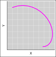
|
| |
| Figure 53: Curved Motion in Space | Figure 54: Seemingly Straight Motion in Space | |
| Figure 55 makes things more explicit. The magneta curve shows Y versus X, while the red curve shows X versus T and the blue curve shows Y versus T. We can see that X is a non-straight function of T, and also Y is a non-straight function of T. | Similarly, figure 56 is unambiguous. The particle is evidently accelerating in a straight line through space. When we look at it in spacetime, we see that X is a non-straight function of T, and also Y is a non-straight function of T. The dots in all these curves are equally spaced in time, which is another way of visualizing the time-dependence. |
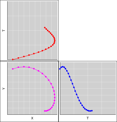
|
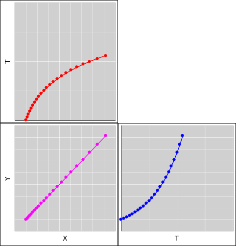
| |
| Figure 55: Curved Motion in Spacetime | Figure 56: Straight in Space, Curved in Spacetime | |
We can visualize things even more clearly using interactive computer graphics.
| The left diagram shows a free particle, following a truly straight path through spacetime. | The right diagram shows the same physical situation as in figure 56. The magenta dots show what’s really going on in (x, y, t) spacetime, in two spacelike dimensions plus one timelike dimension. The gray dots are not real; they are just the shadow, i.e. the projection onto the (x,y) plane, which is a contour of constant t=0. Similarly the light-blue dots are the projection of the motion onto the t axis, which is a contour of constant x and y. You can see that the dots are equally spaced in time. |
| This particle’s true motion – the spacetime motion – is curved, even though the two-dimensional shadow is straight. We conclude that this is not a free particle, because its motion through spacetime is not straight. |
The spacetime viewpoint gives us a very simple, very elegant statement of the first law of motion: A free particle moves in a straight line through spacetime.
We should take the hint: All physics is spacetime physics.
Tangential remark: We use straight-line motion to recognize free particles. We do not need free particles to define what we mean by straight. There is a perfectly good, fundamental geometrical definition of straight, as explained in reference 17.
English translation, from reference 18:
Shut yourself up with some friend in the main cabin below decks on some large ship, and have with you there some flies, butterflies, and other small flying animals. Have a large bowl of water with some fish in it; hang up a bottle that empties drop by drop into a wide vessel beneath it. With the ship standing still, observe carefully how the little animals fly with equal speed to all sides of the cabin. The fish swim indifferently in all directions; the drops fall into the vessel beneath; and, in throwing something to your friend, you need throw it no more strongly in one direction than another, the distances being equal; jumping with your feet together, you pass equal spaces in every direction. When you have observed all these things carefully (though doubtless when the ship is standing still everything must happen in this way), have the ship proceed with any speed you like, so long as the motion is uniform and not fluctuating this way and that. You will discover not the least change in all the effects named, nor could you tell from any of them whether the ship was moving or standing still. In jumping, you will pass on the floor the same spaces as before, nor will you make larger jumps toward the stern than toward the prow even though the ship is moving quite rapidly, despite the fact that during the time that you are in the air the floor under you will be going in a direction opposite to your jump. In throwing something to your companion, you will need no more force to get it to him whether he is in the direction of the bow or the stern, with yourself situated opposite. The droplets will fall as before into the vessel beneath without dropping toward the stern, although while the drops are in the air the ship runs many spans. The fish in their water will swim toward the front of their bowl with no more effort than toward the back, and will go with equal ease to bait placed anywhere around the edges of the bowl. Finally the butterflies and flies will continue their flights indifferently toward every side, nor will it ever happen that they are concentrated toward the stern, as if tired out from keeping up with the course of the ship, from which they will have been separated during long intervals by keeping themselves in the air. And if smoke is made by burning some incense, it will be seen going up in the form of a little cloud, remaining still and moving no more toward one side than the other. The cause of all these correspondences of effects is the fact that the ship’s motion is common to all the things contained in it, and to the air also. That is why I said you should be below decks; for if this took place above in the open air, which would not follow the course of the ship, more or less noticeable differences would be seen in some of the effects noted.
In the original, from reference 19:
Risserratevi con qualche amico nella maggiore stanza, che sia sotto coverta di alcun gran navilio, e quivi fate d’ aver mosche, farfalle e simili animaletti volanti: siavi anco un gran vaso d’acqua, e dentrovi de’pescetti; sospendasi anco in alto qualche secchiello, che a goccia a goccia vada versando dell’ acqua in un altro vaso di angusta bocca che sia posto a basso; e stando ferma la nave, osservate diligentemente, come quelli animaletti volanti con pari velocità vanno verso tutte le parti della stanza; i pesci si vedranno andar notando inditferentemente per tutti i versi, le stille cadenti entreranno tutte nel vaso sottoposto; e voi gettando all’ amico alcuna cosa, non più gagliardamente la dovrete gettare verso quella parte che verso questa, quando le lontananze sieno eguali; e saltando voi, come si dice, a piè giunti, eguali spazj passerete verso tutte le parti. Osservate che avrete diligentemente tutte queste cose, benchè niun dubbio ci sia che mentre il vascello sta fermo non debbano succeder cosi; fate muover la nave con quanta si voglia velocità: chè (pur che il moto sia uniforme e non fluttuante in qua e in là) voi non riconoscerete una minima mutazione in tutti li nominati effetti; nè da alcuno di quelli potrete comprender se la nave cammina, o pure sta ferma. Voi saltando passerete nel tavolato i medesimi spazj che prima; nè perchè la nave si muova velocissimamente, farete maggior salti verso la poppa, che verso la prora, benchè nel tempo che voi state in aria il tavolato sottopostovi scorra verso la parte contraria al vostro salto; e gettando alcuna cosa al compagno, non con più forza bisognerà tirarla per arrivarlo, se egli sarà verso la prora e voi verso poppa, che se voi fuste situati per l’ opposito: le gocciole cadranno come prima nel vaso inferiore senza caderne pur una verso poppa, benchè, mentre la gocciola è per aria, la nave scorra molti palmi; ipesci nella lor acqua non con più fatica noteranno verso la precedente che verso la susseguente parte del vaso; ma con pari agevolezza verranno al cibo posto su qualsivoglia luogo dell’ orlo del vaso; e finalmente le farfalle e le mosche continueranno i lor voli indifferentemente verso tutte le parti; nè mai accederà che si riduchino verso la parete che riguarda la poppa, quasi che fussero stracche in tener dietro al veloce corso della nave, dalla quale per lungo tempo trattenendosi per aria saranno state separate: e se, abbruciando alcuna lagrima d’ incenso, si farà un poco di fumo, vedrassi ascender in alto, e a guisa di nugoletta trattenervisi, e indifferentemente muoversi non più verso questa che quella parte: e di tutta questa corrispondenza d’ efletti ne è cagione l’ esser il moto della nave comune a tutte le cose contenute in essa, e all’aria ancora; che perciò dissi io che si stesse sotto coverta, chè quando si stesse di sopra e nell’aria aperta e non seguace del corso della nave, differenze più e men notabili si vedrebbero in alcuni degli effetti nominati.
| | ||||
| Henceforth, space of itself and time of itself | ||||
| shall sink into mere shadows | ||||
| and only a kind of union of the two | ||||
| shall maintain its independence. | ||||
| | ||||
| Or in the original: | ||||
| | ||||
| | Von Stund’ an sollen Raum für sich und Zeit für sich | | ||
| völlig zu Schatten herabsinken | ||||
| und nur noch eine Art Union der beiden | ||||
| soll Selbständigkeit bewahren. | ||||
| | ||||
| ||||
That must be one of the most profound sentences in human history. The notion of time as the fourth dimension is a serious, powerful, quantitative idea. It is not some loose, hand-wavy metaphor. It is not science fiction.
When doing anything involving special relativity, very often the first step is to draw the spacetime diagram. Draw a grid consisting of unit-spaced contours of constant x running in one direction, along with unit-spaced contours of of constant t running in another direction. Then plot the events relative to the grid. Contours are incomparably better than axes, for reasons discussed in reference 21. The geometry of spacetime is just enough different from the familiar Euclidean geometry that you shouldn’t guess what the grid looks like. Construct a quantitatively correct grid, perhaps using the techniques outlined in section 7.3.
The separation between two events is a four-vector. To measure the gorm of this four-vector – or any other four-vector – you can use the grid to find the spacetime coordinates. Then you can calculate the gorm mathematically.
A more pictorial approach is to construct a frame in which the four-vector of interest is purely timelike (or purely spacelike). Then you can use the grid in this frame as a ruler, and simply count how many contours of constant t (or constant x) are crossed by the vector.
Beware that you cannot measure distance by any other kind of ruler, or by eye, for reasons discussed in section 7.2. In general, you cannot safely use a draftsman’s compass, dividers, or an ordinary ruler to measure a physically-significant distance on a spacetime diagram. To repeat: The only safe way to use a ruler is to make sure the vector is purely timelike (or purely spacelike) in some frame, and then use a ruler that is calibrated for that frame, including the gamma-factor appropriate to that frame.
Keep in mind that the spacetime diagram is not an entirely faithful representation. On the other hand, an imperfect representation is better than no representation. As mentioned in section 4.17 in connection with figure 34, you have to be a bit careful about how you measure time and distance in the red frame, if you are not at rest in that frame. Here is a copy of the diagram:
| Let the coordinates on the paper itself be (u, v). |
| Suppose the paper is being used to represent real-world spacelike coordinates (x, y). Then the geometry of the paper is a reasonably faithful representation of the real geometry. | Suppose the paper (u, v) is being used to represent real-world spacetime coordinates (t, x). Then the geometry of the paper is not an entirely faithful representation of the real geometry. |
| In particular, distances on the paper are in one-to-one correspondence to the real-world distances. | Distances on the paper are not in one-to-one correspondence with the real-world spacetime intervals. |
| In the real (x, y) plane, the gorm is the squared distance, namely x2 + y2. It is always positive. It is closely analogous to the squared distance in the plane the paper, namely u2 + v2. | In the (t, x) plane, the gorm is x2 − t2, with an important minus sign. The gorm is positive in some directions and negative in other directions. This is quite unlike the squared distance in the plane of the paper, namely u2 + v2. |
| As a conspicuous example, consider a light ray that is emitted at one point and absorbed at another point. The world-line of the light ray covers a nonzero distance in the (u, v) plane, even though the corresponding spacetime interval is zero. |
| Distances in the (x, y) plane are invariant with respect to rotation, and the (u, v) plane exhibits the same invariance. | Distances and intervals in the (t, x) plane are invariant with respect to rotations – including boosts – but distances in the (u, v) plane are not. |
| As another way of saying the same thing: In typical Cartesian representations of Euclidean space, the lines of constant x are perpendicular to the lines of constant y. Therefore, if the lines in some given set of lines “look” close together, they are. | On a spacetime diagram, in any frame where the axes are tilted, that frame’s lines of constant t will meet the t axis at a shallow angle. Therefore lines that “look” close together might in fact be spread out over a large amount of frame-time in that frame. This is the “evening shadow” effect. |
The best way to defend against these limitations is to draw the grids; not just an axis or two, but the full grids, as discussed in section 7.1. This gives you a systematic, misconception-resistant way of finding the coordinates of any event.
| You presumably find it easy to draw a rotated coordinate system, provided the rotation is spacelike and confined to the xy plane, such as we see in figure 44. You have seen thousands upon thousands of rotated objects in your lifetime. | When you get to the point where you have seen thousands of spacetime diagrams, including boosted coordinate systems, you will be able draw them freehand ... but until then, it is probably easier and better to use prefabricated spacetime graph paper, or to create your own using a computer. |
Some prefabricated spacetime graph paper is available online; see e.g. reference 22.
If you want to make your own, here are some suggestions:
Keep a safe copy of this file. You will need it more than once.
This results in a quantitatively-correct boost.
Since we have not set the E and F matrix elements, the boosted object will probably get moved to a strange place, so you will have to find it and move it back to wherever it belongs.
As an alternative: You can create drawings in LATEX, using the “tikz” package. For an example, see reference 23.
Another suggestion: It is usually better to rotate text using a simple spacelike rotation, rather than a boost, because a boost would give the text a sheared look and make it hard to read. If a coordinate system has undergone a boost of angle θ, its labels should undergo a spacelike rotation of angle atan(tanh(θ)). Note that here we are using the hyperbolic tanh function and the circular atan function. We leave it as an exercise to prove that this is the correct angle.
And another: If there is any chance that you will ever want a complex diagram such as figure 28, draw it first. Then if you want a simplified view of the same situation, you can prepare it by copying the complicated drawing and deleting everything you don’t need. The point here is that deleting stuff from a complicated drawing obviously preserves alignment, whereas every time you add stuff to a simple diagram you have to fuss with the alignment.
In particular: The drawing program has a layers feature. You may find it advantageous to use one layer for the fundamental physics (spacetime events and four-vectors), another layer for the red reference frame, and another layer for the blue reference frame, and so on. You can then selectively make layers visible or invisible.
Also, the layer locking feature comes in handy. Locking the grid layers allows you to drag stuff relative to the grid, with no risk of accidentally dragging the grid.
My diagrams gradually improve over time. I do all my editing on the complicated diagram, and use the makefile mechanism to derive the various simplified views automatically. This reduces my workload while guaranteeing that consistency will be maintained. Hint: You can assign names to graphical objects, which makes it easy for the makefile to select them for deletion.
Knowing a few trig identities is useful when thinking about relativity. It is especially useful when reading the literature, because it helps you recognize and simplify some otherwise-scary-looking expressions. Let’s start with the basic Pythagorean identity:
| In figure 59, the red bar represents the base b, the blue bar represents the altitude a, and the green curve is a circle representing the locus of constant b2 + a2. | In figure 60, the red bar represents the base b, the blue bar represents the altitude a, and the green curve is a hyperbola representing the locus of constant b2 − a2. |
| In both figures, the small black circles mark angles, from 0 to 1 radian inclusive, in steps of 1/4 radian. |
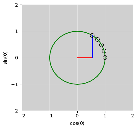
|
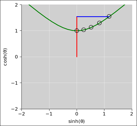
| |
| Figure 59: Circular Trigonometry | Figure 60: Hyperbolic Trigonometry | |
| The corresponding trig identity is: | The corresponding hyperbolic trig identity has an important minus sign: |
| Let’s be explicit about the corresondences: |
|
|
|||||||||||||||||||||||||||||||
| It is also useful to be able to convert back and forth between trig functions and exponentials. These are particularly useful for deriving the double-angle identities: |
|
|
| From these, we can derive lots more identities. We can use these identities to simplify physics problems. For example: |
| Suppose an object is moving along an upward-sloping path. We are given the slope s. We want to calculate the ratio between the actual length of the path and the ground track, i.e. the projection of the path onto the laboratory x-axis. One reasonable approach is to do it in two steps: Take the arctangent of the slope to find the angle θ, and then take the cosine of θ in the usual way. | Let’s revisit the muon-lifetime experiment discussed in section 4.11. The muon is moving along at a certain velocity relative to the lab frame. We prefer to think of this in terms of its four-velocity u, but alas the Muggle we hired as a lab assistant only measured the reduced velocity v as seen in the lab frame. We want to calculate the ratio between the muon’s actual elapsed time (proper time!) and the projection of its time onto the laboratory t-axis. Recall that this projection factor dt/dτ is conventionally called γ. One reasonable approach is to do it in two steps, as we did in section 4.11: Take the hyperbolic arctangent of the reduced velocity to find the rapidity θ, and then take the hyperbolic cosine of θ in the usual way. |
| If we do this often enough, we might want a shortcut, i.e. a formula to go from slope to projection-factor in one step. Such a formula is provided by equation 99c. It is easy to derive this formula whenever you need it, as follows: | If we do this often enough, we might want a shortcut, i.e. a formula to go from reduced velocity to gamma-factor in one step. Such a formula is provided by equation 100c. It is easy to derive this formula whenever you need it, as follows: |
| Let’s recall some terminology. Using the same a, b, and c as in the Pythagorean equation 89, we can express the slope as: | Let’s recall some terminology: The reduced velocity is: |
| We start with equation 91 and divide through by the first term. | We start with equation 92 and divide through by the first term. |
|
|
| We see that the projection factor cos(⋯) is always less than or equal to 1. When the slope is small, the projection factor is unity, and as the slope goes to infinity, the projection factor goes to zero, in accordance with equation 99c. | We see that the projection factor cosh(⋯) is always greater than or equal to 1. When the velocity is small, the projection factor is unity, and as the velocity approaches the speed of light, the projection factor diverges to infinity, in accordance with equation 100c. |
| Another way of writing the cosine can be obtained by re-arranging equation 89. | Another way of writing the hyperbolic cosine can be obtained by re-arranging equation 90. |
|
|
There is not any deep physics in any of this. These are little more than trigonometric identities. Equation 99c tells us about the cosine of the arctangent, while equation 101 tells us about the cosine of the arcsine.
Beware: All too often, discussions of special relativity have a great many formulas that involve factors of 1/√(1−v2/c2). However, you should avoid this as much as possible. If you are ever tempted to write such a thing, you should consider writing something else instead, something more elegant, something with more direct physical significance, such as γ or cosh(θ) or dt/dτ. Expressing the factor in terms of v puts too much emphasis on v, which is an old-fashioned three-dimensional quantity. You will gain more insight if you express the factor in terms of spacetime quantities such as four-vectors or Lorentz scalars.
If we are interested in momentum, we should always start with the definition in equation 10. Here it is again:
| (103) |
That is the best model we have for the physics of the universe we live in, namely the physics of spacetime. Starting from this simple, elegant, powerful formula, we can always make things more complicated and more restricted if necessary. For example, suppose we have a particle (such as a muon) moving through the laboratory. Before it decays, it gets absorbed by something. We know the mass, and our lab assistant has measured the reduced velocity v. We want a one-step formula that tells us how much momentum the particle imparts to the absorber. We can easily derive such a formula:
|
Equation 104h is useful in specialized situations, but obviously it is messier, less fundamental, and more restricted than equation 103. Here’s the recommended strategy:
For an example of what can go wrong if you skip the first steps in this process, and use equation 104h as your starting point, see reference 11.
Again: Beware that it is not a good idea to put too much emphasis on expressions involving v. It is better to focus attention on legitimate four-vectors and Lorentz scalars, because they communicate more about what is actually going on in spacetime. If you are given a 3-vector, usually the best strategy is to convert it to the corresponding spacetime vector as quickly as possible. Learn to think in four dimensions.
Let’s do one more example: Suppose we know where the particle is initially, and we want to know where it will be a short time later. That’s simple:
| (105) |
Equation 105 is a clear expression of a simple concept. It is obviously correct, as a corollary of the definition of velocity, equation 71. Here is the definition again:
| (106) |
As always, the recommended strategy is to remember the simple formulas, namely equation 105 and equivalently equation 71. These are so simple and so obviously consistent with grade-school notions of “distance equals rate times time” that they are hard to forget. You can complexify things later, if the situation warrants.
For example, suppose we want to find where the particle will be a short time later, but for some reason we choose to express this in terms of “time” as measured by laboratory clocks ... not the particle’s proper time. We know the mass, and our lab assistant has measured the three spatial components of the momentum, pxyz. Note that measuring the momentum is smarter than measuring the velocity, especially if the velocity is near the speed of light.
The physics here is simple, if we think about it in spacetime. We know the four-momentum of the particle in its own rest frame, namely p = [mc, 0, 0, 0]. The momentum is purely timelike in that frame. When the particle is moving relative to the lab frame, the four-momentum gets rotated. A piece of its four-momentum gets projected onto the spacelike directions in the lab frame. This projection is the blue bar in figure 60, as mentioned in equation 94. It is what we measure as the particle’s pxyz in the lab frame. The relevant projection factor is sinh(θ), as we have seen in equation 53 and elsewhere.
We can use this, plus a trig identity, to obtain a useful expression for gamma:
| (107) |
Equation 107 is sometimes useful, because it expresses γ in terms of the 3-momentum pxyz, which can sometimes be relatively easy to measure. This equation is a cousin to equation 100c, which expresses γ in terms of the reduced velocity v; however, beware that equation 107 has a plus sign inside the square root, whereas equation 100c has a minus sign.
We can apply this idea to the “distance equals rate times time” equation.
|
Equation 108i is useful in special situations. Its advantage is that the RHS involves only things that Muggles can measure: three-dimensional momentum, wall-clock time, et cetera. Another alleged advantage is that it involves only algebraic math functions, not transcendental trig functions. The disadvantage is that it is ugly, messy, and hard to remember. This is the penalty you pay for thinking in terms of pre-1908 three-dimensional concepts.
In contrast, equation 105 is a clear expression of a simple concept. It is vastly clearer than equation 108i. It is also 33% more powerful, because it gives us all four spacetime components, not just the three spacelike components. It is the nice, simple, modern (post-1908) way to represent the physics. It is obviously correct, as a corollary of the definition of velocity, equation 71.
In practice, you do not need equation 108i. The recommended alternative is simple: Whenever you get a three-vector, convert it to the corresponding four-vector as soon as possible. Even if you wind up converting back to three-vectors at the end of the calculation, the extra work is negligible, and the advantage in terms of conceptual clarity is overwhelming. Along these lines, note that having an algebraic formula (as in equation 108h) offers no practical advantage over the transcendental trigonometric formula (as in equation 108f). Every “scientific” pocket calculator made in the 20 or 30 years can do hyperbolic trig functions just as easily as it can do square roots.
In any case, comparing equation 105 to equation 108i tells us a lot about what’s going on. Both have the structure of “distance equals rate times time”. Equation 108i has a factor of 1/γ out front, because we decided to measure wall-clock time (Δt) rather than proper time (Δτ), but other than that, the formulas are the same. If somebody shows you equation 108i by surprise, the main barrier to understanding it is recognizing that the first factor is just a messy way of expressing 1/γ.
This document takes a modern (post-1908) approach to the subject. Alas, there are a great many other documents in the world that seem to think that the development of relativity began and ended in 1905. This results in some exceedingly confusing concepts, as well as some needlessly ugly equations.
If at all possible, you should avoid exploring the unwise ways of doing things. It just pollutes your brain. You’ve been warned. However, if you dare to ignore this warning, and if you want to see how horrible the un-modern approach can be, see reference 11.
Remember, though: In most cases, the less said about such things, the better. For all practical purposes, there is nothing you need to know about pre-1908 relativity. The modern approach is easier and in every way better.