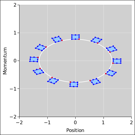
Figure 1: Phase Space of a Harmonic Oscillator
Liouville’s theorem says that area in phase space is conserved. This is one of the most fundamental results in theoretical physics. Unlike the more familiar laws such as conservation of energy, momentum, and charge, it does not apply to some region in ordinary space that you have chosen. Instead, it applies to the region in an abstract space mapped out by a collection of particles, all moving subject to the same equation of motion, with different initial conditions. The region may change shape, as shown in figure 1, but the area stays the same.
This theorem is exceedingly fundamental. It applies to the quantum-mechanical world, and carries over without change in the classical approximation. All of the following are intimately connected; a violation of any one could be used to construct a violation of the others:
It’s also analogous to Feistel ciphers.
Note that the dynamical phase space were are talking about here has got nothing to do with the “phase space” that shows up in thermodynamics and physical chemistry. Nothing to do with the Gibbs phase rule.
Let’s start by considering a specific system, and see what the laws of physics (including Liouville’s theorem) have to say about it. We choose the simple case of particles moving in circular orbits in a gravitational field. Here are some technical details:
There are 9 particles. The red group in figure 2 is a snapshot of the particles at the initial time, t0. Two of the nine particles have been colored black, but they are still considered part of the red group. The green group in the figure is a snapshot of the particles at a later time, t1. Similarly, the blue group is a snapshot of the particles at an even later time, t2.
You can see that the group does not maintain its shape as it moves along. This is because the particles in the small-ρ orbits move faster while the particles in large-ρ orbits move slower, in accordance with the three laws of motion, Kepler’s laws, and all the other laws of physics.
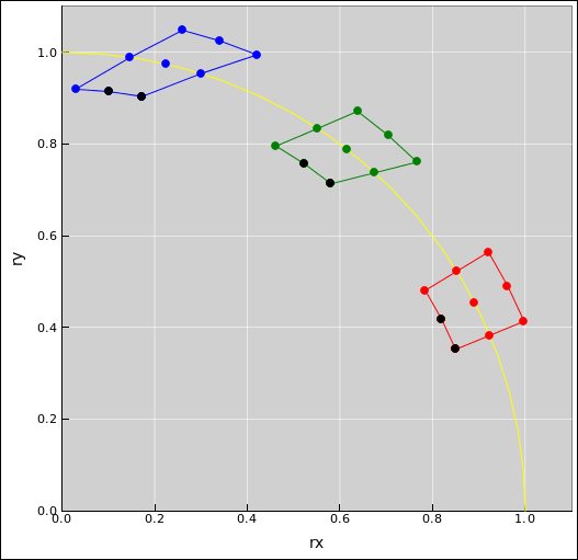
As each particle goes around in its orbit, its radius-vector r changes with time, and also its momentum p changes in time. The momentum behaves as shown in figure 3. As before, red corresponds to time t0, green corresponds to time t1, and blue corresponds to time t2.
By comparing this figure to the previous figure, you see that the particles with the largest |r| have the smallest |p|, and vice versa. Hint: Look at the black dots.
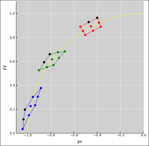
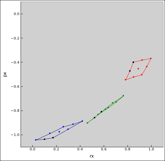
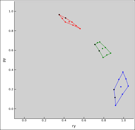
Things get much more interesting if we plot position against momentum (rather than position against position, or momentum against momentum). We do this separately for each of the N dimensions. The plot of the x-component of momentum against the x-component of the radius vector is shown in figure 4. Similarly the plot of the y-component of momentum against the y-component of the radius vector is shown in figure 5.
|
| |
| Figure 4: Circular Orbits : Flow in Phase Space (x) | Figure 5: Circular Orbits : Flow in Phase Space (y) | |
It is interesting to look at the «area» in phase space occupied by our group of particles. Actually it’s not really an area in the Euclidean sense, but rather a bivector in the Clifford Algebra sense. If you’re not familiar with bivectors, to a good approximation you can cross out the word bivector every time you see it and replace it with the word “area” – but keep in mind that it is an oriented area. Just as two vectors can have the same length but different direction, two bivectors can have the same area and different orientation. In two dimensions, we reckon the bivector as negative or positive, depending on whether we go around the boundary in the clockwise or counterclockwise direction (respectively). (For details on bivectors and such things, see reference 2.)
To determine the orientation for each group in figure 4 and similar diagrams, start at the black dot that sits on a corner. Then proceed to the adjacent black dot that sits in the middle of a side. Then continue in that direction. For example, as shown in figure 4, as time progresses from red to green to blue, the rxpx-contribution to the total bivector-value progresses from positive to nearly zero to negative.
This is interesting because if, at each time, you add the bivectors in figure 4 to the bivectors in in figure 5, the result is the same at all times. In particular:
The spreadsheet that produces these figures is also programmed to measure the bivectors. The total is constant over time, to an accuracy of one part in 1014, which is almost as accurately as the spreadsheet can compute anything.
Liouville’s theorem proves that the total bivector is always constant, for any system. Specifically:
For any group of points, the total bivector (in phase space) occupied by the group remains unchanged over time, as the group flows along in accordance with the laws of motion.
I mention the following items without explaining them, because explaining them would require explaining almost all of physics.
It is important to understand what Liouville’s theorem is telling us ... and also to understand what it is not telling us.
It might tell us what is going on in the neighborhood of a single point, as in section 5 ... but the existence of a neighborhood, by definition, depends on the existence of additional points in the neighborhood.
See section 6 for more on this.
Note that many introductory discussions of Liouville’s theorem emphasize a one-dimensional system (such as a harmonic oscillator) to the near-exclusion of multi-dimensional systems. This is unfortunate, becaue the multi-dimensional behavior is richer, in ways that cannot be guessed based on the one-dimensional behavior. Specifically:
To say the same thing another way, phase space itself is 2N-dimensional, but the thing that matters to Liouville’s theorem is a grade=2 bivector, regardless of N.
There are various ways to determine the magnitude and direction of the relevant bivectors. In introductory calculus you learned to find the area of the curve as
| (1) |
assuming you know how to express the boundary of the region in terms of a function p(r) ... which is sometimes convenient and sometimes not.
Similarly, if you turn your head 90 degrees you can write
| (2) |
More generally, we can express the bivector of group g as the two-dimensional integral
| (3) |
where Ig is an indicator function that tells whether or not we are inside the group. In addition, Ig needs to account for negative versus positive orientation, depending on whether the boundary is oriented clockwise versus counterclockwise ... which means that actually using equation 3 is a bit tricky.
The three previous equations apply to a one-dimensional system, such as a harmonic oscillator. More generally, for an N-dimensional system, we need to evaluate the total bivector.
| (4) |
Here is a highly questionable argument: Liouville’s theorem says that the S in equation 4 is unchanging over time. If we claim that this is true for any function Ig, then we conclude that dri dpi itself must be unchanging over time. However, that claim is false, because equation 4 is only valid provided Ig flows in accordance with the laws of motion. In fact, equation 4 tells us more about Ig than it does about dri or dpi.
I mention this because you sometimes see Liouville’s theorem stated in terms of dri dpi, as if that were the whole story. Experts know there are some hugely important provisos that go along with such a statement, whereas non-experts are completely mystified.
Also note that dri dpi is often written as dri ∧ dpi, using a wedge product. However, if you construct things such that dri is perpendicular to dpi, then dri dpi is equivalent to dri ∧ dpi, so we don’t need to worry about it. Actually, it’s even worse than that, as you can see from the warnings associated with equation 7.
Things are even simpler if the region of interest in phase space is a polygon, or can be well approximated by a polygon. Any polygon can be divided into triangles. If we consider the bivector defined by points A, B, and C in a 2-dimensional phase space, its magnitude and direction are given by:
| (5) |
For a system with N dimensions, i.e. a 2N-dimensional phase space, the total bivector is:
| (6) |
Note that in equation 6 I passed up the opportunity to write the “elegant” (but wrong) expression
| (7) |
That is wrong because the bivectors (as constructed by the wedge product) have direction as well as magnitude. As surely as one coordinate r1 is perpendicular to another coordinate r2, the bivector r1 ∧ p1 is perpendicular to the bivector r2 ∧ p2. If the bivectors were coplanar, equation 6 would be the correct way to add them, but they are not, so it isn’t.
There may be an elegant-and-correct geometrical interpretation of equation 6, but if so, I don’t know about it. I do know that the interpretation in terms of bivectors is not correct. By the same token, any interpretation in terms of cross products is not correct.
Let’s ask: What is the physical significance of the orientation of the various bivectors? Suppose the total bivector-value is S = S1 + S2 + ⋯. Then there are two answers:
It’s a fluke of 2D that it’s even possible to label bivectors as positive or negative. In any higher dimensional space, we would have to talk about direction more generally.
It’s analogous to vectors in 1D: by a fluke we can classify them as positive or negative. In contrast, in two or more dimensions a vector can’t be called positive or negative; all you can do is specify a direction, such as north by northeast ... and even that is relative to some chosen basis, and the choice of basis cannot possibly have any physical significance.
For bivectors in 2D, the sign depends on choosing the right-hand rule versus the left-hand rule. Equivalently, it involves choosing a way of ordering the basis vectors. Strictly speaking, the basis shouldn’t be called a basis «set», because it’s really an ordered list of basis vectors.
Here’s another way of stating Liouville’s theorem:
The laws of motion require the probability density in phase space to exhibit continuity of flow. The probability is locally conserved.
Here, flow means just what you think it means, in analogy to the flow of in indestructible incompressible fluid. For more on this, see reference 4.
This is equivalent to the formulation given at the end of section 2, as we can see from the following argument: We represent the probability density in phase space by constructing points, such that the density of points (per unit area) represents the probability density. Then we have one formulation that quantifies the area of the points, and another that quantifies points per unit area. If one of those quantities is unchanging then the other is unchanging.
Here we are using the fact that the points themselves are indestructible. We know that is true, because the entire future (and past) motion of the system is determined by the current radius-vector r and momentum-vector p. Therefore points in phase space cannot split (or merge).
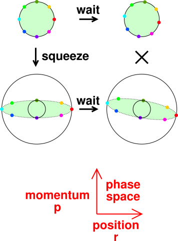
Figure 6 shows four snapshots of the phase space of a harmonic oscillator. In particular, we imagine a pendulum consisting of a point-mass at the end of a string. The color-code in this figure is different from previously. Sorry about that.
The axes in phase space are, as always, the radius-vector r and the momentum p, where r and p are canonically conjugate.
We start with the upper-left snapshot. This shows an ensemble of 8 harmonic oscillators. They all have the same energy. They have 8 different phases, evenly distributed, as shown.
The equation of motion says that each and every oscillator follows a circular path in phase space. So they play follow-the-leader around the circle. The upper-right diagram shows the situation if we take a snapshot 1/36th of a cycle after the upper-left snapshot. Everything is rotated 10 degrees.
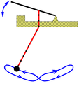
Things get more interesting if we modulate the length of the string in accordance with the scheme diagrammed in figure 7.
Specifically, as indicated by the figure-8 in figure 7, we lengthen the string at the end of each half-cycle, and then we shorten the string at the middle of each half cycle (doing work against centrifugal force). We do this gradually but persistently. For any oscillator that has the “right” phase relative to the phase of the pump, we add energy to the system, as shown by e.g. the red and cyan dots in the phase-space diagram, i.e. the dots that start out at the 3:00 and 9:00 positions. On the other hand,for any oscillator that has the “wrong” phase, we suck energy out of the system, as shown by e.g. the dark green and dark blue dots, i.e. the dots that start out at the 12:00 and 6:00 positions. If we perform such pumping on an ensemble of oscillators, after a while we get a new ensemble, as shown by the lower-left snapshot.
We now discontinue the parametric pumping.
Note that the bivector defined by the ensemble of oscillators (as shown by the light green shading) is invariant with respect to the parametric pumping operation. The initially circular distribution of oscillators has become an ellipse, as shown in the lower-left snapshot. The new distribution is 2x smaller in the p direction and 2x larger in the q direction ... so the bivector is the same.
This is an example of a Bogoliubov transformation. That is, essentially we have just redefined the units on the q axis and redefined the units on the p axis to match, so that the new p and q are canonically conjugate. If this doesn’t mean anything to you, don’t worry about it.
As always, the equation of motion tells us that each oscillator rotates around the origin in phase space. The lower-right snapshot shows a snapshot 1/36th of a cycle later than the lower-left snapshot.
You can find lots of references that claim E/ω is invariant, for any particular oscillator, when it undergoes an adiabatic transformation.
This claim is very, very wrong, as you can see from the example in figure 6. For some members of the ensemble, E increased very substantially, while for other members, E decreased very substantially. All that is without any significant change in ω. At all times the parametric modulation was small and infinitely differentiable.
Let’s be clear: Note the contrast:
See reference 1.