Beware: In the thermodynamics literature, the word “state” is used with two inconsistent meanings. It could mean either microstate or macrostate.
| In a system such as the deck of cards discussed in section 2.3, the microstate is specified by saying exactly which card is on top, exactly which card is in the second position, et cetera. | In that system, the macrostate is the ensemble of all card decks consistent with what we know about the situation. |
| In a system such as a cylinder of gas, a microstate is a single fully-specified quantum state of the gas. | For such a gas, the macrostate is specified by macroscopic variables such as the temperature, density, and pressure. |
| In general, a macrostate is an equivalence class, i.e. a set containing some number of microstates (usually many, many microstates). |
| In the context of quantum mechanics, state always means microstate. | In the context of classical thermodynamics, state always means macrostate, for instance in the expression “function of state”. |
The idea of microstate and the idea of macrostate are both quite useful. The problem arises when people use the word “state” as shorthand for one or both. You can get away with state=microstate in introductory quantum mechanics (no thermo), and you can get away with state=macrostate in introductory classical thermo (no quantum mechanics) … but there is a nasty collision as soon as you start doing statistical mechanics, which sits astride the interface between QM and thermo.
| In this document, the rule is that state means microstate, unless the context requires otherwise. | When we mean macrostate, we explicitly say macrostate or thermodynamic state. The idiomatic expression “function of state” necessarily refers to macrostate. |
The relationship between microstate and macrostate, and their relationship to entropy, is discussed in section 2.7 and section 12.1.
Also, chapter 20 is a tangentially-related discussion of other inconsistent terminology.
Remember that the entropy is a property of the macrostate, not of any particular microstate. The macrostate is an ensemble of identically-prepared systems.
Therefore, if you are studying a single system, the second law doesn’t necessarily tell you what that system is going to do. It tells you what an ensemble of such systems would do, but that’s not necessarily the same thing. At this point there are several options. The ensemble average is the strongly recommended option.
Note that energy is well defined for a single microstate but entropy is not. Entropy is a property of the macrostate. You may wish for more information about the microstate, but you won’t get it, not from the second law anyway.
Given a probability distribution:
| You can find the mean of the distribution. | However, the mean does not tell you everything there is to know. |
| You can find the standard deviation of the distribution. | However, the standard deviation does not tell you everything there is to know. |
| You can find the entropy of the distribution. | However, the entropy does not tell you everything there is to know. |
| Even those three things together do not tell you everything there is to know. |
Note that distribution = ensemble = macrostate. The literature uses three words that refer to the same concept. That’s annoying, but it’s better than the other way around. (Using one word for three different concepts is a recipe for disaster.)
Suppose we have some source distribution, namely a distribution over some N-dimensional vector X. This could represent the positions and momenta of N/6 atoms, or it could represent something else. Now suppose we draw one point from this distribution – i.e. we select one vector from the ensemble. We call that the sample. We can easily evaluate the sample-mean, which is just equal to the X-value of this point. We do not expect the sample-mean to be equal to the mean of the source distribution. It’s probably close, but it’s not the same.
Similarly we do not expect the sample-entropy to be the same as the source-distribution-entropy. Forsooth, the entropy of the sample is zero!
Given a larger sample with many, many points, we expect the sample-entropy to converge to the source-distribution-entropy, but the convergence is rather slow.
The discrepancy between the sample-mean and the source-dist-mean is not what people conventionally think of as a thermodynamic fluctuation. It’s just sampling error. Ditto for the sample- entropy versus the source-dist-entropy. Fluctuations are dynamic, whereas you get sampling error even when sampling a distribution that has no dynamics at all. For example, given an urn containing colored marbles, the marbles are not fluctuating ... but different samples will contain different colors, in general.
For more about the crucial distinction between a distribution and a point drawn from that distribution, see reference 1, especially the section on sampling.
As mentioned in section 2.5.2, our notion of entropy is completely dependent on having a notion of microstate, and on having a procedure for assigning probability to microstates.
For systems where the relevant variables are naturally discrete, this is no problem. See section 2.2 and section 2.3 for examples involving symbols, and section 11.10 for an example involving real thermal physics.
We now discuss the procedure for dealing with continuous variables. In particular, we focus attention on the position and momentum variables.
It turns out that we must account for position and momentum jointly, not separately. That makes a lot of sense, as you can see by considering a harmonic oscillator with period τ: If you know the oscillator’s position at time t, you know know its momentum at time t+τ/4 and vice versa.
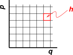
Figure 12.1 shows how this works, in the semi-classical approximation. There is an abstract space called phase space. For each position variable q there is a momentum variable p. (In the language of classical mechanics, we say p and q are dynamically conjugate, but if you don’t know what that means, don’t worry about it.)
Area in phase space is called action. We divide phase space into cells of size h, where h is Planck’s constant, also known as the quantum of action. A system has zero entropy if it can be described as sitting in a single cell in phase space. If we don’t know exactly where the system sits, so that it must be described as a probability distribution in phase space, it will have some correspondingly greater entropy.
If you are wondering why each state has area h, as opposed to some other amount of area, see section 26.10.
If there are M independent position variables, there will be M momentum variables, and each microstate will be associated with a 2M-dimensional cell of size hM.
Using the phase-space idea, we can already understand, qualitatively, the entropy of an ideal gas in simple situations:
For a non-classical variable such as spin angular momentum, we don’t need to worry about conjugate variables. The spin is already discrete i.e. quantized, so we know how to count states … and it already has the right dimensions, since angular momentum has the same dimensions as action.
In chapter 2, we introduced entropy by discussing systems with only discrete states, namely re-arrangements of a deck of cards. We now consider a continuous system, such as a collection of free particles. The same ideas apply.
For each continuous variable, you can divide the phase space into cells of size h and then see which cells are occupied. In classical thermodynamics, there is no way to know the value of h; it is just an arbitrary constant. Changing the value of h changes the amount of entropy by an additive constant. But really there is no such arbitrariness, because “classical thermodynamics” is a contradiction in terms. There is no fully self-consistent classical thermodynamics. In modern physics, we definitely know the value of h, Planck’s constant. Therefore we have an absolute scale for measuring entropy.
As derived in section 26.2, there exists an explicit, easy-to-remember formula for the molar entropy of a monatomic three-dimensional ideal gas, namely the Sackur-Tetrode formula:
| = ln( |
| ) + |
| (12.1) |
where S/N is the molar entropy, V/N is the molar volume, and Λ is the thermal de Broglie length, i.e.
| Λ := √( |
| ) (12.2) |
and if you plug this Λ into the Sackur-Tetrode formula you find the previously-advertised dependence on h3.
You can see directly from equation 26.17 that the more spread out the gas is, the greater its molar entropy. Divide space into cells of size Λ3, count how many cells there are per particle, and then take the logarithm.
The thermal de Broglie length Λ is very commonly called the thermal de Broglie wavelength, but this is something of a misnomer, because Λ shows up in a wide variety of fundamental expressions, usually having nothing to do with wavelength. This is discussed in more detail in reference 35.
Imagine a crystal of pure copper, containing only the 63Cu isotope. Under ordinary desktop conditions, most of the microscopic energy in the crystal takes the form of random potential and kinetic energy associated with vibrations of the atoms relative to their nominal positions in the lattice. We can find “normal modes” for these vibrations. This is the same idea as finding the normal modes for two coupled oscillators, except that this time we’ve got something like 1023 coupled oscillators. There will be three normal modes per atom in the crystal. Each mode will be occupied by some number of phonons.
At ordinary temperatures, almost all modes will be in their ground state. Some of the low-lying modes will have a fair number of phonons in them, but this contributes only modestly to the entropy. When you add it all up, the crystal has about 6 bits per atom of entropy in the thermal phonons at room temperature. This depends strongly on the temperature, so if you cool the system, you quickly get into the regime where thermal phonon system contains much less than one bit of entropy per atom.
There is, however, more to the story. The copper crystal also contains conduction electrons. They are mostly in a low-entropy state, because of the exclusion principle, but still they manage to contribute a little bit to the entropy, about 1% as much as the thermal phonons at room temperature.
A third contribution comes from the fact that each 63Cu nucleus can be be in one of four different spin states: +3/2, +1/2, -1/2, or -3/2. Mathematically, it’s just like flipping two coins, or rolling a four-sided die. The spin system contains two bits of entropy per atom under ordinary conditions.
You can easily make a model system that has four states per particle. The most elegant way might be to carve some tetrahedral dice … but it’s easier and just as effective to use four-sided “bones”, that is, parallelepipeds that are roughly 1cm by 1cm by 3 or 4 cm long. Make them long enough and/or round off the ends so that they never settle on the ends. Color the four long sides four different colors. A collection of such bones is profoundly analogous to a collection of copper nuclei. The which-way-is-up variable contributes two bits of entropy per bone, while the nuclear spin contributes two bits of entropy per atom.
In everyday situations, you don’t care about this extra entropy in the spin system. It just goes along for the ride. This is an instance of spectator entropy, as discussed in section 12.6.
However, if you subject the crystal to a whopping big magnetic field (many teslas) and get things really cold (a few millikelvins), you can get the nuclear spins to line up. Each nucleus is like a little bar magnet, so it tends to align itself with the applied field, and at low-enough temperature the thermal agitation can no longer overcome this tendency.
Let’s look at the cooling process, in a high magnetic field. We start at room temperature. The spins are completely random. If we cool things a little bit, the spins are still completely random. The spins have no effect on the observable properties such as heat capacity.
As the cooling continues, there will come a point where the spins start to line up. At this point the spin-entropy becomes important. It is no longer just going along for the ride. You will observe a contribution to the heat capacity whenever the crystal unloads some entropy.
You can also use copper nuclei to make a refrigerator for reaching very cold temperatures, as discussed in section 11.10.
Some people who ought to know better try to argue that there is more than one kind of entropy.
Sometimes they try to make one or more of the following distinctions:
| Shannon entropy. | Thermodynamic entropy. |
| Entropy of abstract symbols. | Entropy of physical systems. |
| Entropy as given by equation 2.2 or equation 27.6. | Entropy defined in terms of energy and temperature. |
| Small systems: 3 blocks with 53 states, or 52 cards with 52! states | Large systems: 1025 copper nuclei with 41025 states. |
It must be emphasized that none of these distinctions have any value.
For starters, having two types of entropy would require two different paraconservation laws, one for each type. Also, if there exist any cases where there is some possibility of converting one type of entropy to the other, we would be back to having one overall paraconservation law, and the two type-by-type laws would be seen as mere approximations.
Also note that there are plenty of systems where there are two ways of evaluating the entropy. The copper nuclei described in section 11.10 have a maximum molar entropy of R ln(4). This value can be obtained in the obvious way by counting states, just as we did for the small, symbol-based systems in chapter 2. This is the same value that is obtained by macroscopic measurements of energy and temperature. What a coincidence!
Let’s be clear: The demagnetization refrigerator counts both as a small, symbol-based system and as a large, thermal system. Additional examples are mentioned in chapter 22.
Suppose we define a bogus pseudo-entropy S′ as
| S′ := S + K (12.3) |
for some arbitrary constant K. It turns out that in some (but not all!) situations, you may not be sensitive to the difference between S′ and S.
For example, suppose you are measuring the heat capacity. That has the same units as entropy, and is in fact closely related to the entropy. But we can see from equation 7.14 that the heat capacity is not sensitive to the difference between S′ and S, because the derivative on the RHS annihilates additive constants.
Similarly, suppose you want to know whether a certain chemical reaction will proceed spontaneously or not. That depends on the difference between the initial state and the final state, that is, differences in energy and differences in entropy. So once again, additive constants will drop out.
There are many standard reference books that purport to tabulate the entropy of various chemical compounds … but if you read the fine print you will discover that they are really tabulating the pseudo-entropy S′ not the true entropy S. In particular, the tabulated numbers typically do not include the contribution from the nuclear spin-entropy, nor the contribution from mixing the various isotopes that make up each element. They can more-or-less get away with this because under ordinary chem-lab conditions those contributions are just additive constants.
However, you must not let down your guard. Just because you can get away with using S′ instead of S in a few simple situations does not mean you can get away with it in general. As discussed in section 12.7 there is a correct value for S and there are plenty of cases where the correct value is needed.
Suppose we want to find the value of the true entropy, S. We account for the thermal phonons, and the electrons, and the nuclear spins. We even account for isotopes, chemical impurities, and structural defects in the crystal. But … how do we know when to stop? How do we know if/when we’ve found all the entropy? In section 12.6 we saw how some of the entropy could silently go along for the ride, as a spectator, under certain conditions. Is there some additional entropy lurking here or there? Could there be hitherto-unimagined quantum numbers that couple to hitherto-unimagined fields?
The answer is no. According to all indications, there is no secret entropy. At any temperature below several thousand degrees, electrons, atomic nuclei, and all other subatomic particles can be described by their motion (position and momentum) and by their spin, but that’s it, that’s a complete description. Atoms, molecules, and all larger structures can be completely described by what their constituent particles are doing.
In classical mechanics, there could have been an arbitrary amount of secret entropy, but in the real world, governed by quantum mechanics, the answer is no.
We have a firm experimental basis for this conclusion. According to the laws of quantum mechanics, the scattering of indistinguishable particles is different from the scattering of distinguishable particles.
Therefore let’s consider a low-energy proton/proton scattering experiment. We arrange that the protons are not distinguishable on the basis of position, or on any basis other than spin. That is, the protons are indistinguishable if and only if they have the same spin.
Next we randomize the spins, so that for each proton, each of the two spin states is equally likely. Our ignorance of the spin state contributes exactly 1 bit per particle to the entropy.
Now, to make things interesting, suppose that in addition to the aforementioned 1 bit of spin-entropy, each proton had 17 bits of “secret entropy”, in whatever form you can imagine. That would mean that there would be 217 different distinguishable types of proton. If you pick protons at random, they would almost certainly be distinguishable, whether or not their spins were aligned, and you would almost never observe like-spin scattering to be different from unlike-spin scattering.
Such scattering experiments have been conducted with electrons, protons, various heavier nuclei, and sometimes entire atoms. There has never been any indication of any secret entropy.
The thermodynamics of chemical reactions tells us that larger structures can be described in terms of their constituents with no surprises.
The existence of superfluidity is further evidence that we can correctly account for entropy. All the atoms in the superfluid phase are described by a single quantum wavefunction. The entropy per atom is zero; otherwise it wouldn’t be a superfluid. Superfluid 4He depends on the fact that all 4He atoms are absolutely totally indistinguishable – not distinguishable on the basis of position, spin, or any other quantum numbers. This is what we expected, based on two-particle scattering experiments, but the existence of superfluidity reassures us that we haven’t overlooked anything when going from two particles to 1023 particles.
Superfluidity occurs because certain identical-particle effects are cumulative and therefore have a spectacular effect on the entire fluid. Similar macroscopic identical-particle effects have been directly observed in 3He, spin-polarized monatomic hydrogen, sodium atomic gas, and other systems.
It might also be remarked that the existence of superconductors, semiconductors, metals, molecular bonds, and the periodic table of elements is strong evidence that electrons have no secret entropy. The existence of lasers is strong evidence that photons have no secret entropy.
I can’t prove that no hitherto-secret entropy will ever be discovered. We might discover a new atom tomorrow, called loonium, which is exactly the same as helium except that for some reason it always obeys the distinguishable-particle scattering law when scattering against helium. This wouldn’t be the end of the world; we would just postulate a new quantum number and use it to distinguish the two types of atom. All I can say is that loonium must be exceedingly rare; otherwise it would have been noticed.
Reminder: The foregoing discussion applies to “secret entropy” that might exist at room temperature or below, in analogy to spin entropy. In contrast we are not talking about the plethora of quantum numbers that are known to come into play at higher energies, but are all in their ground state under ordinary room-temperature conditions.
Consider 100 decks of cards. The first one is randomly shuffled. It has an entropy of just under 226 bits. All the rest are ordered the same way as the first. If you give me any one of the decks in isolation, it will take me 226 yes/no questions to figure out how to return the deck to standard order. But after I’ve seen any one of the decks, I know the exact microstate of every other deck without asking additional questions. The other 99 decks contain zero additional entropy.
In a situation like this, it’s hard to consider entropy to be a state variable. In particular, the entropy density will not be an intensive property.
I know this sounds creepy, but it’s real physics. Creepy situations like this do not usually occur in physical systems, but sometimes they do. Examples include:
In an ordinary ideal gas, you can pretty much assume the entropy density is a well-behaved intensive property – but don’t completely let down your guard, or you’ll be badly fooled by the spin-echo setup.
A related issue concerns the dependence of entropy on the choice of observer. Entropy is not simply a property of a system, but rather a property of the system and the description thereof. This was mentioned in passing near the end of chapter 2.
Let’s be clear: As a matter of principle, two different observers will in general assign two different values to “the” entropy.
This is easy to express in mathematical terms. The trustworthy workhorse formula for entropy is equation 2.2. If we have a conditional probability, things get slightly more complicated, as discussed in section 12.9.
Human observers are so grossly dissipative and usually “know” so little that it is academic to worry about the thermodynamics of human “knowledge”. However, the issue takes on new life when we consider tiny, highly-optimized robot measuring devices – Maxwell demons and the like.
For microscopic systems, it is for sure possible for different observers to report different values of “the” entropy (depending on what each observer knows about the system). The discrepancy can be a large percentage of the total.
By way of analogy, you know that different observers report different values of “the” kinetic energy (depending on the velocity of the observer), and this hasn’t caused the world to end.
For macroscopic systems (1023 particles or thereabouts) it is uncommon for one observer to know 1023 things that the other observer doesn’t … but even this is possible. The spin echo experiment is a celebrated example, as discussed in section 11.7.
Regardless of the size of the system, it is often illuminating to consider a complete thermodynamic cycle, such that all participants are returned to the same state at the end of the cycle. This de-emphasizes what the observers “know” and instead focuses attention on how they “learn” … and how they forget. In more technical terms: this focuses attention on the observation/measurement process, which is crucial if you want a deep understanding of what entropy is and where it comes from. See reference 36 and reference 37.
In particular, at some point in each cycle the observer will have to forget previous information, to make room for the new information. This forgetting expels entropy, and at temperature T it dissipates energy TS.
To repeat: When evaluating “the” entropy, it is necessary to account for the information in the observer-system. In a closed cycle, this focuses attention on the observation and measurement process. If you don’t do this, you will get the wrong answer every time when analyzing spin echo systems, Maxwell demons, Szilárd engines, reversible computers, et cetera.
Suppose we have the following joint probability:
| (12.4) |
From that we can form the marginal probabilities such as u=a+b and v=c+d:
| (12.5) |
To allow for the possibility that the probabilities are not normalized, we define
| (12.6) |
The conditional probabilities (conditioned on row number) are:
| (12.7) |
Notation: The probability is conditioned on the variable marked with the “@” sign, as discussed in reference 1. Briefly, we can define this notation in terms of the older “|” bar notation:
| (12.8) |
Then for each row y, we can define the row entropy:
| (12.9) |
So in our example, the row entropy of the first row is:
| (12.10) |
An analogous expression exists for the column entropy. The term slice entropy is meant to encompass row entropy, column entropy, and all other ways of slicing up the joint distribution. If the probability is a function of N variables, there will be 2N−2 ways of slicing things.
We can now define the full-blown conditional entropy as the weighted sum of the row entropies:
| (12.11) |
So in our example, the conditional entropy is:
| (12.12) |
Note that the row entropy is a function of row number, but the full conditional entropy is not. Both of them are, of course, a functional of the probability distribution.
In this section, we consider three possibilities:
Calculating the entropy of an extreme mixture is a bit tricky. It may help to use playing cards as a model system. There are two possible scenarios:
Next we shuffle the cards within the hand, so that we no longer know the order of the cards. Now there is 2.6 bits of entropy, i.e. log2(3!).
Note: In this section, all numerical values for the entropy are rounded to the nearest 0.1 bit.
Let’s call this the entropy of permutation of the hand. For some purposes we might consider this “the” entropy, but not for all purposes, as we shall see. As another way of saying the same thing: we have just calculated a row entropy (as defined in section 12.9 – conditioned on knowing which three cards are in the hand.
In this example, S|D is just the entropy of permutation within the hand. (For another system, such as a sample of gas, we would need a more complicated expression for S|D.)
Very commonly, the entropy of the deal is enormous compared to the entropy if permutation within the hand.
In general, the total system entropy is
| (12.13) |
Reminder: The entropy of the deal, by definition, does not include the entropy of permutation within the sample.
Under mild conditions, the number of possible deals will be:
| (12.14) |
where WD is the multiplicity of the deal, M is the number of particles in the universal set, and N is the number of particles that were selected (dealt) into the actual sample. Here we are assuming that the particles, although distinguishable, all behave very nearly the same, so that they have equal probability of being selected.
When the number of particles in the universal set (cards in the deck) is very large compared to the number of particles actually in the sample, equation 12.14 simplifies to:
| (12.15) |
We now consider a two-handed version of the same game. Once again, there are two scenarios, depending on whether we peek or not.
Next, we put the two hands together and shuffle the six cards. Now the system entropy is 9.5 bits, i.e. log2(6!).
The main result here is that the system entropy is increased by mixing the two subsystems. It has gone up from 5.2 to 9.5, for a gain of 4.3 bits. This newly created entropy, called the entropy of mixing, can be considered a minature entropy of the deal, created by dealing two hands from the six-card mini-deck.
We now turn to an ugly and messy side-issue, which you can skip if you want. If we re-separate these card into two hands of three, it is not easy to decide how the system entropy gets distributed. Each player, considering his hand alone, evalutes the entropy as 6.9 bits, i.e. log2(6*5*4), since he doesn’t know which three of the six cards he’s got, or what order they’re in. That leaves the familiar 2.6 bits in the other player’s hand.
This is another example of context-dependent entropy, as discussed in section 12.8. By symmetry, each player evaluates the entropy of his own hand as 6.9 bits and the entropy of the other player’s hand as 2.6 bits. Each of these evaluations is consistent with itself, but not consistent with the other evaluation.
Immediately after dealing the cards, the system entropy is 33.8 bits, i.e. log2(52*51*50*49*48*47). If the cards were dealt in the usual way, we can say this entropy is distributed as follows: There is 16.9 bits in the first hand hand, i.e. log2(52*50*48), plus 16.8 bits in the other hand, i.e. log2(51*49*47).
Next, we put the two hands together and shuffle the six cards. This does not increase the entropy. Before the shuffling, we knew nothing about which six cards were involved and knew nothing about the order, and after the shuffling we don’t know any more or less. The system entropy is still 33.8 bits.
The main result is that in this scenario, mixing does not increase the entropy.
Once again we have a messy and ugly side issue: We now re-separate the cards into two hands of three. It is, alas, tricky to decide how the entropy is distributed. It might make sense to distribute the entropy evenly, by symmetry. Or it might make sense to say it was distributed as before, namely 16.9 plus 16.8. Or it might make sense for one player to decide that in the absence of information about the other player’s hand, he should use the maximally-asymmetric worst-case estimate, namly 17 bits in his hand, i.e. log2(51*51*50), plus 16.8 bits in the other hand i.e. log2(49*48*47).
Note the contrast:
In scenario 2A, mixing increased the entropy. This can be explained by saying that we zeroed out the entropy of the deal by peeking, and then re-created a little bit of entropy of the deal by shuffling the six-card mini-deck and re-dealing.
In scenario 2B, mixing did not increase the entropy. The system already had the maximal amount of entropy of the deal, so shuffling the mini-deck and re-dealing could not possibly increase the entropy.
We now consider a contrast along a different axis, namely the contrast between a pure substance and an extreme mixture:
| For a sample of helium, the entropy of the deal is zero. That’s because all 4He atoms are identical. One sample of N atoms of helium is just like any other sample of N atoms of helium. | For a sample of gas where the particles are all different, like the proverbial snowflakes, the total entropy necessarily includes the entropy of the deal. If you have N snowflakes, in general it matters which N snowflakes they are. If you have two such samples, each individual flake is different, and each sample as a whole is different. The two samples may be equivalent as to various macroscopic average properties, but from the point of view of the foundations of thermodynamics, the two samples are very different. They are different in a way that two samples of helium are not. |
| If we perform a Gibbs-type mixing experiment with helium, mixing does not increase the entropy. This makes sense, because all helium atoms are identical. |
If we perform a Gibbs-type mixing experiment with snow, there are two
possibilities. In scenario 2A (as discussed in
section 12.10.2), mixing increases the entropy. In
this scenario the entropy of the deal had been removed, and mixing
re-created a certain amount of entropy of the deal. Meanwhile, in scenario 2B, mixing does not increase the entropy. |
Note that the non-increase of entropy for mixing snow in scenario 2B is not equivalent to the non-increase for mixing helium; they occur for different reasons.
There is yet another scenario that is worth considering, namely where we have only partial information about the particles in each sample. Roughly speaking, imagine mixing red snow with blue snow, or mixing chocolate milk with regular milk.
Again we use playing cards as our model system.
The information about the coloration of each hand can be considered partial information. This information could come from any of several possible sources, including a weak peek, i.e. a peek that ascertains the color without ascertaining the exact suit or rank.
If we put the two hands together and shuffle the six cards, the system entropy increases to 32.2 bits, which breaks down as 22.7 for the entropy of the original deal (unchanged), plus 9.5 for the entropy of permutation of the six cards, i.e. log2(6!). So the entropy-gain due to mixing is 4.3 bits.
Not coincidentally, this is the exact-same entropy gain as we saw in scenario 2A. The change is the same, even though the system entropy of the new scenario (2C) is greater. In both of these scenarios, the entropy of mixing is associated with not knowing which of the two original hands contributed a given card to the final hand.
Again it is tricky to distribute the system entropy. If each player adopts the worst-case maximum entropy strategy, he will attribute 17.0 bits of entropy to his hand, i.e. log2(52*51*50), since he really has no idea what cards are in his hand. This leaves 15.2 bits in the other hand. This is another situtaion where each player’s evaluation is internally consistent, but inconsistent with the other player’s evaluation.
People commonly think of entropy as being an extensive quantity. This is true to a good approximation in many situations, especially for macroscopic systems in thermal equilibrium. However, there are exceptions.
As an extreme example of non-extensive entropy, consider the situation described at the beginning of section 12.8, where we have one randomly-shuffled deck plus some number of clones. Whichever one of these decks we look at first will look completely random, but the total entropy of the system does not grow in proportion to the number of decks; indeed it does not grow at all as we add more decks.
Even for something as simple as a pure monatomic ideal gas, the entropy is “almost” extensive, but not quite, as discussed in connection with equation 26.17. Similarly, for a gas mixture, see equation 26.21.
The idea that entropy might be non-extensive should not come as any big surprise. The energy of a liquid or solid is not exactly extensive either, because of things like surface tension and surface reconstruction.
Note that in a Gibbs-type mixing experiment, if you start out with helium on one side and neon on the other, the entropy of the mixture is not the sum of the two original entropies. Not even close. This is because there is a large entropy of mixing. In this situation we might say the entropy is grossly non-extensive (if it even makes sense to talk about extensivity in such a situation).
On the other hand, if we start out with a mixture of helium and neon on one side, and the same mixture on the other side, when we pull out the partition, there is “almost” no change in entropy, in accordance with equation 26.21.
Similarly, even for an extreme mixture, i.e. snow on one side and snow on the other, the entropy is extensive (or nearly so) ... provided we account for the entropy of the deal. Beware that the entropy of the deal is often neglected, even though it is enormous.
Let’s see what it takes to construct a probability distribution that has infinite entropy.
For simplicity, let’s consider a discrete distribution, with discrete microstates ... such as a distribution over the integers. (A continuous distribution would make the problem more complicated but not in any way more interesting.)
There are two ways to proceed. Let’s deal with the simple, not-so-interesting case first. Imagine tossing a very large number of coins. The entropy per coin (s) is intensive and is the same everywhere, namely 1 bit per coin. The total entropy (S) is extensive, and grows in proportion to the number of coins. This situation is easy to understand in the case of a large but finite number of coins, but things go haywire if we ask about a truly infinite number of coins, because then there would be an infinite number of microstates with zero probability apiece. Zero probability is not good.
We can apply the same logic to the physics of a large chunk of metal. The molar entropy, s, is intensive and is the same everywhere. The total entropy, S, is extensive and grows in proportion to the size of the chunk. Again, this is easy to understand for a large but finite chunk, but things to haywire if we ask about a truly infinite chunk, because then every microstate would have zero probability.
So let’s not approach the problem that way. Instead we insist on a well behaved probability distribution, such that
where j is some convenient starting-point. The goal of infinite entropy means that
| (12.17) |
Finding a suitable distribution is going to be a challenge, because we want the series in equation 12.16b to converge, but we want the closely-related series in equation 12.17 to diverge. This is possible, but it means that one series will “just barely” converge while the other will “just barely” diverge.
Let’s see whether the probability defined by equation 12.18 does what we want.
| (12.18) |
As an aid to understanding what’s going on, consider the series in equation 12.19. Using the integral test, you can easily show that the series converges for all h strictly greater than 1, and diverges to +∞ otherwise.
| (12.19) |
Returning to equation 12.18, let’s assume h is greater than one. For definiteness, you can take h=1.5 if you wish. This guarantees that the probability is well-behaved as specified in equation 12.16.
We can calculate a lower bound on the entropy as follows:
| (12.20) |
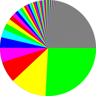
The pie chart for this distribution is shown (somewhat impefectly) in figure 12.2. You can see that the series converges quite slowly. In fact, the first 1000 terms cover only about 86% of the total pie when h=2.0. Smaller values of h give even slower convergence.
I can’t think of any physics situations where there are countably many states, each with a positive amount of probability ... but such situations are routine in data compression, communications, and cryptography. It’s an argument for having variable-length codewords. There are infinitely many different messages that could be sent. A few of them are very common and should be encoded with short codewords, while most of the rest are very very unlikely, and should be encoded with much longer codewords.
This is a way of driving home the point that entropy is a property of the distribution.
The idea of entropy applies to any distribution, not just thermal-equilibrium distributions.
Here is another example of a countable, discrete distribution with infinite entropy:
| (12.21) |
This has the advantage that we can easily calculate the numerical value of Z. If you approximate this distribution using a Taylor series, you can see that for large i, this distribution behaves similarly to the h=2 case of equation 12.18. This distribution is discussed with more formality and more details in reference 38.