The second law of thermodynamics states that entropy obeys a local paraconservation law. That is, entropy is “nearly” conserved. By that we mean something very specific:
| (2.1) |
The structure and meaning of equation 2.1 is very similar to equation 1.1, except that it has an inequality instead of an equality. It tells us that the entropy in a given region can increase, but it cannot decrease except by flowing into adjacent regions.
As usual, the local law implies a corresponding global law, but not conversely; see the discussion at the end of section 1.2.
Entropy is absolutely essential to thermodynamics … just as essential as energy. The relationship between energy and entropy is diagrammed in figure 0.1. Section 0.1 discusses the relationship between basic mechanics, information theory, and thermodynamics. Some relevant applications of entropy are discussed in chapter 22.
Entropy is defined and quantified in terms of probability, as discussed in section 2.6. In some situations, there are important connections between entropy, energy, and temperature … but these do not define entropy; see section 2.5.7 for more on this. The first law (energy) and the second law (entropy) are logically independent.
If the second law is to mean anything at all, entropy must be well-defined always. Otherwise we could create loopholes in the second law by passing through states where entropy was not defined.
Entropy is related to information. Essentially it is the opposite of information, as we see from the following scenarios.
As shown in figure 2.1, suppose we have three blocks and five cups on a table.
To illustrate the idea of entropy, let’s play the following game: Phase 0 is the preliminary phase of the game. During phase 0, the dealer hides the blocks under the cups however he likes (randomly or otherwise) and optionally makes an announcement about what he has done. As suggested in the figure, the cups are transparent, so the dealer knows the exact microstate at all times. However, the whole array is behind a screen, so the rest of us don’t know anything except what we’re told.
Phase 1 is the main phase of the game. During phase 1, we (the players) strive to figure out where the blocks are. We cannot see what’s inside the cups, but we are allowed to ask yes/no questions, whereupon the dealer will answer. Our score in the game is determined by the number of questions we ask; each question contributes one bit to our score. The goal is to locate all the blocks using the smallest number of questions.
Since there are five cups and three blocks, we can encode the location of all the blocks using a three-symbol string, such as 122, where the first symbol identifies the cup containing the red block, the second symbol identifies the cup containing the black block, and the third symbol identifies the cup containing the blue block. Each symbol is in the range zero through four inclusive, so we can think of such strings as base-5 numerals, three digits long. There are 53 = 125 such numerals. (More generally, in a version where there are N cups and B blocks, there are NB possible microstates.)
To calculate what our score will be, we don’t need to know anything about energy; all we have to do is count states (specifically, the number of accessible microstates). States are states; they are not energy states.
Superficially speaking, if you wish to make this game seem more thermodynamical, you can assume that the table is horizontal, and the blocks are non-interacting, so that all possible configurations have the same energy. But really, it is easier to just say that over a wide range of energies, energy has got nothing to do with this game.
The point of all this is that we can measure the entropy of a given situation according to the number of questions we have to ask to finish the game, starting from the given situation. Each yes/no question contributes one bit to the entropy, assuming the question is well designed. This measurement is indirect, almost backwards, but it works. It is like measuring the volume of an odd-shaped container by quantifying the amount of water it takes to fill it.
The central, crucial idea of entropy is that it measures how much we don’t know about the situation. Entropy is not knowing.
Here is a card game that illustrates the same points as the cup game. The only important difference is the size of the state space: roughly eighty million million million million million million million million million million million states, rather than 125 states. That is, when we move from 5 cups to 52 cards, the state space gets bigger by a factor of 1066 or so.
Consider a deck of 52 playing cards. By re-ordering the deck, it is possible to create a large number (52 factorial) of different configurations.
Technical note: There is a separation of variables. We choose to consider only the part of the system that describes the ordering of the cards. We assume these variables are statistically independent of other variables, such as the spatial position and orientation of the cards. This allows us to understand the entropy of this subsystem separately from the rest of the system, for reasons discussed in section 2.8.Also, unless otherwise stated, we assume the number of cards is fixed at 52 ... although the same principles apply to smaller or larger decks, and sometimes in an introductory situation it is easier to see what is going on if you work with only 8 or 10 cards.
Phase 0 is the preliminary phase of the game. During phase 0, the dealer prepares the deck in a configuration of his choosing, using any combination of deterministic and/or random procedures. He then sets the deck on the table. Finally he makes zero or more announcements about the configuration of the deck.
Phase 1 is the main phase of the game. During phase 1, we (the players) strive to fully describe the configuration, i.e. to determine which card is on top, which card is second, et cetera. We cannot look at the cards, but we can ask yes/no questions, whereupon the dealer will answer. Each question contributes one bit to our score. Our objective is to ascertain the complete configuration using the smallest number of questions. As we shall see, our score is a measure of the entropy of the game.
Note the contrast between microstate and macrostate:
| One configuration of the card deck corresponds to one microstate. The microstate does not change during phase 1. | The macrostate is the ensemble of microstates consistent with what we know about the situation. This changes during phase 1. It changes whenever we obtain more information about the situation. |
At this point we know that the deck is in some microstate, and the microstate is not changing … but we don’t know which microstate. It would be foolish to pretend we know something we don’t. If we’re going to bet on what happens next, we should calculate our odds based on the ensemble of possibilities, i.e. based on the macrostate.
Our best strategy is as follows: By asking six well-chosen questions, we can find out which card is on top. We can then easily describe every detail of the configuration. Our score is six bits.
This illustrates that the entropy is a property of the ensemble, i.e. a property of the macrostate, not a property of the microstate. Cutting the deck the second time changed the microstate but did not change the macrostate. See section 2.4 and especially section 2.7.1 for more discussion of this point.
Note that we are not depending on any special properties of the “reference” state. For simplicity, we could agree that our reference state is the factory-standard state (cards ordered according to suit and number), but any other agreed-upon state would work just as well. If we know deck is in Moe’s favorite state, we can easily rearrange it into Joe’s favorite state. Rearranging it from one known state to to another known state does not involve any entropy.
As a variation on the game described in section 2.3, consider what happens if, at the beginning of phase 1, we are allowed to peek at one of the cards.
In the case of the standard deck, example 1, this doesn’t tell us anything we didn’t already know, so the entropy remains unchanged.
In the case of the cut deck, example 3, this lowers our score by six bits, from six to zero.
In the case of the shuffled deck, example 6, this lowers our score by six bits, from 226 to 220.
This is worth mentioning because peeking can (and usually does) change the macrostate, but it cannot change the microstate. This stands in contrast to cutting an already-cut deck or shuffling an already-shuffled deck, which changes the microstate but does not change the macrostate. This is a multi-way contrast, which we can summarize as follows:
| Macrostate Changes | Macrostate Doesn’t Change | |||||
| Microstate Usually Changes: |
|
| ||||
| Microstate Doesn’t Change: |
|
|
This gives us a clearer understanding of what the macrostate is. Essentially the macrostate is the ensemble, in the sense that specifying the ensemble specifies the macrostate and vice versa. Equivalently, we can say that the macrostate is a probability distribution over microstates.
In the simple case where all the microstates are equiprobable, the ensemble is simply the set of all microstates that are consistent with what you know about the system.
In a poker game, there is only one deck of cards. Suppose player Alice has peeked but player Bob has not. Alice and Bob will then play according to very different strategies. They will use different ensembles – different macrostates – when calculating their next move. The deck is the same for both, but the macrostate is not. This idea is discussed in more detail in connection withf figure 2.4 in section 2.7.2.
We see that the physical state of the deck does not provide a complete description of the macrostate. The players’ knowledge of the situation is also relevant, since it affects how they calculate the probabilities. Remember, as discussed in item 4 and in section 2.7.1, entropy is a property of the macrostate, not a property of the microstate, so peeking can – and usually does – change the entropy.
To repeat: Peeking does not change the microstate, but it can have a large effect on the macrostate. If you don’t think peeking changes the ensemble, I look forward to playing poker with you!
The models we have been discussing are in some ways remarkably faithful to reality. In some ways they are not merely models but bona-fide examples of entropy. Even so, the entropy in one situation might or might not convey a good understanding of entropy in another situation. Consider the following contrasts:
| Small Model Systems | More Generally |
| We have been considering systems with only a few bits of entropy (the cup game in section 2.2) or a few hundred bits (the card deck in section 2.3). | In the physics lab or the chemistry lab, one might be dealing with 100 moles of bits. A factor of 6×10²³ can have significant practical consequences. |
| Entropy is defined in terms of probability. Entropy is not defined in terms of energy, nor vice versa. There are plenty of situations where the second law is important, even though the temperature is irrelevant, unknown, and/or undefinable. | In some (albeit not all) practical situations there is a big emphasis on the relationship between energy and temperature, which is controlled by entropy. |
| There are some experiments where it is possible to evaluate the entropy two ways, namely by counting the bits and by measuring the energy and temperature. The two ways always agree. Furthermore, the second law allows us to compare the entropy of one object with the entropy of another, which provides strong evidence that all the entropy in the world conforms to the faithful workhorse expression, namely equation 2.2, as we shall see in section 2.6. |
| We have been asking yes/no questions. Binary questions are required by the rules of the simple games. | Other games may allow more general types of questions. For example, consider the three-way measurements in reference 13. |
| The answer to each yes/no question gives us one bit of information, if the two answers (yes and no) are equally likely. | If the two answers are not equally likely, the information will be less. |
| So far, we have only considered scenarios where all accessible microstates are equally probable. In such scenarios, the entropy is the logarithm of the number of accessible microstates. | If the accessible microstates are not equally probable, we need a more sophisticated notion of entropy, as discussed in section 2.6. |
| Remark on terminology: Any microstates that have appreciable probability are classified as accessible. In contrast, microstates that have negligible probability are classified as inaccessible. Their probability doesn’t have to be zero, just small enough that it can be ignored without causing too much damage. |
| Thermodynamics is a very practical subject. It is much more common for some probability to be negligible than to be strictly zero. |
| In order to identify the correct microstate with confidence, we need to ask a sufficient number of questions, so that the information contained in the answers is greater than or equal to the entropy of the game. |
If you want to understand entropy, you must first have at least a modest understanding of basic probability. It’s a prerequisite, and there’s no way of getting around it. Anyone who knows about probability can learn about entropy. Anyone who doesn’t, can’t.
Our notion of entropy is completely dependent on having a notion of microstate, and on having a procedure for assigning a probability to each microstate.
In some special cases, the procedure involves little more than counting the accessible (aka “allowed”) microstates, as discussed in section 9.6. This type of counting corresponds to a particularly simple, flat probability distribution, which may be a satisfactory approximation in special cases, but is definitely not adequate for the general case.
For simplicity, the cup game and the card game were arranged to embody a clear notion of microstate. That is, the rules of the game specified what situations would be considered the “same” microstate and what would be considered “different” microstates. Note the contrast:
| Our discrete games provide a model that is directly and precisely applicable to physical systems where the physics is naturally discrete, such as systems involving only the nonclassical spin of elementary particles. An important example is the demagnetization refrigerator discussed in section 11.10. | For systems involving continuous variables such as position and momentum, counting the states is somewhat trickier ... but it can be done. The correct procedure is discussed in section 12.3. |
For additional discussion of the relevance of entropy, as applied to thermodynamics and beyond, see chapter 22.
The point of all this is that the “score” in these games is an example of entropy. Specifically: at each point in the game, there are two numbers worth keeping track of: the number of questions we have already asked, and the number of questions we must ask to finish the game. The latter is what we call the the entropy of the situation at that point.
Remember that the macrostate is the ensemble of microstates. In the ensemble, probabilities are assigned taking into account what the observer knows about the situation. The entropy is a property of the macrostate.
At each point during the game, the entropy is a property of the macrostate, not of the microstate. The system must be in “some” microstate, but generally we don’t know which microstate, so all our decisions must be based on the macrostate.
The value any given observer assigns to the entropy depends on what that observer knows about the situation, not what the dealer knows, or what anybody else knows. This makes the entropy somewhat context-dependent. Indeed, it is somewhat subjective. Some people find this irksome or even shocking, but it is real physics. For a discussion of context-dependent entropy, see section 12.8.
Note that entropy has been defined without reference to temperature and without reference to heat. Room temperature is equivalent to zero temperature for purposes of the cup game and the card game. Arguably, in theory, there is “some” chance that thermal agitation will cause two of the cards to spontaneously hop up and exchange places during the game, but that is really, really negligible.
Non-experts often try to define entropy in terms of energy. This is a mistake. To calculate the entropy, I don’t need to know anything about energy; all I need to know is the probability of each relevant state. See section 2.6 for details on this.
Entropy is not defined in terms of energy, nor vice versa.
In some cases, there is a simple mapping that allows us to identify the ith microstate by means of its energy Êi. It is often convenient to exploit this mapping when it exists, but it does not always exist.
In pop culture, entropy is often associated with disorder. There are even some textbooks that try to explain entropy in terms of disorder. This is not a good idea. It is all the more disruptive because it is in some sense half true, which means it might pass superficial scrutiny. However, science is not based on half-truths.
Small disorder generally implies small entropy. However, the converse does not hold, not even approximately; A highly-disordered system might or might not have high entropy. The spin echo experiment (section 11.7) suffices as an example of a highly disordered macrostate with relatively low entropy.
Before we go any farther, we should emphasize – again – that entropy is a property of the macrostate, not of the microstate. In contrast, to the extent that “disorder” has any definite meaning at all, it is a property of the microstate. Therefore, whatever the “disorder” is measuring, it isn’t entropy. (A similar microstate versus macrostate argument applies to the “energy dispersal” model of entropy, as discussed in section 9.8.) As a consequence, the usual textbook illustration – contrasting snapshots of orderly and disorderly scenes – cannot be directly interpreted in terms of entropy. To get any scrap of value out of such an illustration, the reader must make a sophisticated leap:
| The disorderly snapshot must be interpreted as representative of an ensemble with a very great number of similarly-disorderly microstates. The ensemble of disorderly microstates has high entropy. This is a property of the ensemble, not of the depicted microstate or any other microstate. | The orderly snapshot must be interpreted as representative of a very small ensemble, namely the ensemble of similarly-orderly microstates. This small ensemble has a small entropy. Again, entropy is a property of the ensemble, not of any particular microstate (except in the extreme case where there is only one microstate in the ensemble, and therefore zero entropy). |
To repeat: Entropy is defined as a weighted average over all microstates. Asking about the entropy of a particular microstate (disordered or otherwise) is asking the wrong question. If you know what microstate the system is in, the entropy is zero. Guaranteed.
Note the following contrast:
| Entropy is a property of the macrostate. It is defined as an ensemble average. | Disorder, to the extent it can be defined at all, is a property of the microstate. (You might be better off focusing on the surprisal rather than the disorder, as discussed in section 2.7.1.) |
The number of orderly microstates is very small compared to the number of disorderly microstates. That’s because when you say the system is “ordered” you are placing constraints on it. Therefore if you know that the system is in one of those orderly microstates, you know the entropy cannot be very large.
The converse does not hold. If you know that the system is in some disorderly microstate, you do not know that the entropy is large. Indeed, if you know that the system is in some particular disorderly microstate, the entropy is zero. (This is a corollary of the more general proposition that if you know what microstate the system is in, the entropy is zero. it doesn’t matter whether that state “looks” disorderly or not.)
Furthermore, there are additional reasons why the typical text-book illustration of a messy dorm room is not a good model of entropy. For starters, it provides no easy way to define and delimit the states. Even if we stipulate that the tidy state is unique, we still don’t know how many untidy states there are. We don’t know to what extent a shirt on the floor “here” is different from a shirt on the floor “there”. Since we don’t know how many different disorderly states there are, we can’t quantify the entropy. (In contrast the games in section 2.2 and section 2.3 included a clear rule for defining and delimiting the states.)
Examples of low entropy and relatively high disorder include, in order of increasing complexity:
Technical note: There is a separation of variables, analogous to the separation described in section 2.3. We consider only the part of the system that describes whether the coins are in the “heads” or “tails” state. We assume this subsystem is statistically independent of the other variables such as the position of the coins, rotation in the plane, et cetera. This means we can understand the entropy of this subsystem separately from the rest of the system, for reasons discussed in section 2.8.
Randomize the coins by shaking. The entropy at this point is five bits. If you open the box and peek at the coins, the entropy goes to zero. This makes it clear that entropy is a property of the ensemble, not a property of the microstate. Peeking does not change the disorder. Peeking does not change the microstate. However, it can (and usually does) change the entropy. This example has the pedagogical advantage that it is small enough that the entire microstate-space can be explicitly displayed; there are only 32 = 25 microstates.
Ordinarily, a well-shuffled deck of cards contains 225.581 bits of entropy, as discussed in section 2.3. On the other hand, if you have peeked at all the cards after they were shuffled, the entropy is now zero, as discussed in section 2.4. Again, this makes it clear that entropy is a property of the ensemble, not a property of the microstate. Peeking does not change the disorder. Peeking does not change the microstate. However, it can (and usually does) change the entropy.
Many tricks of the card-sharp and the “magic show” illusionist depend on a deck of cards arranged to have much disorder but little entropy.
There is a long-running holy war between those who try to define entropy in terms of energy, and those who try to define it in terms of disorder. This is based on a grotesquely false dichotomy: If entropy-as-energy is imperfect, then entropy-as-disorder “must” be perfect … or vice versa. I don’t know whether to laugh or cry when I see this. Actually, both versions are highly imperfect. You might get away with using one or the other in selected situations, but not in general.
The right way to define entropy is in terms of probability, as we now discuss. (The various other notions can then be understood as special cases and/or approximations to the true entropy.)
We do not define entropy via dS = dQ/T or anything like that, for multiple reasons. For one thing, as discussed in section 8.2, there is no state-function Q such that dQ = TdS (with perhaps trivial exceptions). Even more importantly, we need entropy to be well defined even when the temperature is unknown, undefined, irrelevant, or zero.
The idea of entropy set forth in the preceding examples can be quantified quite precisely. Entropy is defined in terms of probability.1 For any classical probability distribution P, we can define its entropy as:
| S[P] := |
| Pi log(1/Pi) (2.2) |
where the sum runs over all possible outcomes and Pi is the probability of the ith outcome. Here we write S[P] to make it explicit that S is a functional that depends on P. Beware that people commonly write simply S, leaving unstated the crucial dependence on P.
Equation 2.2 is the faithful workhorse formula for calculating the entropy. It ranks slightly below Equation 27.6, which is a more general way of expressing the same idea. It ranks above various less-general formulas that may be useful under more-restrictive conditions (as in section 9.6 for example). See chapter 22 and chapter 27 for more discussion of the relevance and range of validity of this expression.
Subject to mild restrictions, equation 2.2 applies to physics as follows: Suppose the system is in a given macrostate, and the macrostate is well described by a distribution P, where Pi is the probability that the system is in the ith microstate. Then we can say S is the entropy “of the system”.
Expressions of this form date back to Boltzmann (reference 14 and reference 15) and to Gibbs (reference 16). The range of applicability was greatly expanded by Shannon (reference 17). See also equation 27.6.
Beware that uncritical reliance on “the” observed microstate-by-microstate probabilities does not always give a full description of the macrostate, because the Pi might be correlated with something else (as in section 11.7) or amongst themselves (as in chapter 27). In such cases the unconditional entropy S[P] will be larger than the conditional entropy S[P|Q], and you have to decide which is/are physically relevant.
In the games discussed above, it was convenient to measure entropy in bits, because we were asking yes/no questions. Other units are possible, as discussed in section 9.5.
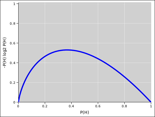
Figure 2.2 shows the contribution to the entropy from one term in the sum in equation 2.2. Its maximum value is approximately 0.53 bits, attained when P(H)=1/e.
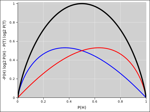
Let us now restrict attention to a system that only has two microstates, such as a coin toss, so there will be exactly two terms in the sum. That means we can identify P(H) as the probability of the the “heads” state. The other state, the “tails” state, necessarily has probability P(T)≡1−P(H) and that gives us the other term in the sum, as shown by the red curve in figure 2.3. The total entropy is shown by the black curve in figure 2.3. For a two-state system, it is necessarily a symmetric function of P(H). Its maximum value is 1 bit, attained when P(H)=P(T)=½.
The base of the logarithm in equation 2.2 is chosen according to what units you wish to use for measuring entropy. Alternatively, as discussed in section 9.5, you can fix the base of the logarithm and stick in a prefactor that has some numerical value and some units:
| S = −k |
| Pi ln Pi (2.3) |
Entropy itself is conventionally represented by big S. Meanwhile, molar entropy is conventionally represented by small s and is the corresponding intensive property.
People commonly think of entropy as being an extensive quantity. This is true to an excellent approximation in typical situations, but there are occasional exceptions. Some exceptions are discussed in section 12.8 and especially section 12.11.
Although it is often convenient to measure molar entropy in units of J/K/mol, other units are allowed, for the same reason that mileage is called mileage even when it is measured in metric units. In particular, sometimes additional insight is gained by measuring molar entropy in units of bits per particle. See section 9.5 for more discussion of units.
When discussing a chemical reaction using a formula such as
| 2 O3 → 3 O2 + Δs (2.4) |
it is common to speak of “the entropy of the reaction” but properly it is “the molar entropy of the reaction” and should be written Δs or ΔS/N (not ΔS). All the other terms in the formula are intensive, so the entropy-related term must be intensive also.
Of particular interest is the standard molar entropy, s∘ i.e. S∘/N, measured at standard temperature and pressure. The entropy of a gas is strongly dependent on density, as mentioned in section 12.3.
If we have a system characterized by a probability distribution P, the surprisal of the ith microstate is given by
| (2.5) |
By comparing this with equation 2.2, it is easy to see that the entropy is simply the ensemble average of the surprisal. In particular, it is the expectation value of the surprisal. (See equation 27.7 for the fully quantum-mechanical generalization of this idea.)
Note the following contrast: For any given microstate i and any given distribution P:
| Surprisal is a property of the microstate i. | Entropy is a property of the distribution P as a whole. It is defined as an ensemble average. |
A manifestation of this can be seen in item 4.
When you hear that entropy is a property of «the» distribution, the word «the» should not receive undue emphasis. The complete assertion says that for any given distribution the entropy is a property of the distribution, and the second half must not be taken out of context. There are lots of different distributions in this world, and you should not think in terms of «the» one true distribution. Indeed, it is common to deal with two or more distributions at the same time.
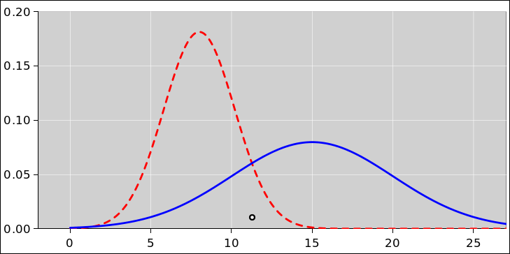
Given just a microstate, you do not know what distribution it was drawn from. For example, consider the point at the center of the small black circle in figure 2.4. The point itself has no uncertainty, no width, no error bars, and no entropy. The point could have been drawn from the red distribution or the blue distribution; you have no way of knowing. The entropy of the red distribution is clearly different from the entropy of the blue distribution.
In a card came such as poker or go fish, it is common for different players to use different macrostates (different distributions), even though the microstate (the objective state of the cards) is the same for all, as discussed in section 2.4. Ditto for the game of Clue, or any other game of imperfect information. Similarly, in cryptography the sender and the attacker virtually always use different distributions over plaintexts and keys. The microstate is known to the sender, whereas the attacker presumably has to guess. The microstate is the same for both, but the macrostate is different.
Another obvious consequence of equation 2.5 is that entropy is not, by itself, the solution to all the world’s problems. Entropy measures a particular average property of the given distribution. It is easy to find situations where other properties of the distribution are worth knowing. The mean, the standard deviation, the entropy, various Rényi functionals, etc. are just a few of the many properties. (Note that the Rényi functionals (one of which is just the entropy) can be defined even in situations where the mean and standard deviation cannot, e.g. for a distribution over non-numerical symbols.)
For more about the terminology of state, microstate, and macrostate, see section 12.1.
Suppose we have subsystem 1 with a set of microstates {(i)} and subsystem 2 with a set of microstates {(j)}. Then in all generality, the microstates of the combined system are given by the direct product of these two sets, namely
| {(i)}×{(j)} = {(i,j)} (2.6) |
where (i,j) is an ordered pair, which should be a familiar idea and a familiar notation. We use × to denote the Cartesian direct product.
We now restrict attention to the less-than-general case where the two subsystems are statistically independent. That means that the probabilities are multiplicative:
| R(i,j) = P(i) Q(j) (2.7) |
Let’s evaluate the entropy of the combined system:
| (2.8) |
where we have used the fact that the subsystem probabilities are normalized.
So we see that the entropy is additive whenever the probabilities are multiplicative, i.e. whenever the probabilities are independent.