|
| |
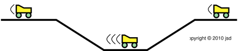
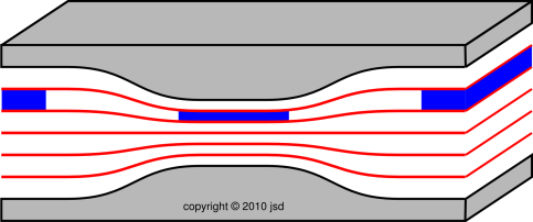
| Figure 1: Roller Coaster | Figure 2: Venturi | |
Bernoulli’s principle is one of the principal results of fluid dynamics.1 It is also known as Bernoulli’s equation or Bernoulli’s theorem. It applies to a particular parcel of fluid as it flows along. In its simplest version it says that when the parcel’s speed decreases the pressure increases and vice versa.
Our discussion will start with the simplest version and progress to more complete, more versatile versions.
There are at least two valid ways of deriving Bernoulli’s equation. An approach based on energy and enthalpy is presented in section 2. An approach based on force, work, and kinetic energy is presented in section 3.
A tabletop apparatus for demonstrating Bernoulli’s principle is described in reference 1.
We consider the behavior of a particular parcel of fluid as it flows along a stream line. We assume the system is non-dissipative; that is, we assume that viscosity and thermal conductivity make a negligible contribution to the energy budget. For simplicity, we assume a steady pressure distribution, although this restriction can easily be lifted, as discussed in section 3.2.
We start by invoking the law of conservation of energy. As always, this law says that any change in the energy within the parcel must be exactly balanced by the transfer of energy across the boundary of the parcel. That is:
| change(energy inside boundary) = − flow(energy, outward across boundary) (1) |
For more on what we mean by “conservation”, see reference 2.
The energy inside the parcel can take various forms, including kinetic energy, gravitational energy, and the energy stored in the “springiness” of the fluid. In a gas such as air, the latter is sometimes called the “thermal” energy, but of course the laws of thermodynamics apply to all forms of energy, not just the air-spring energy. Equation 2 restates what we have just said, expressing it in mathematical terms:
| (2) |
In this section, we use the following symbols:
| (3) |
Be careful to distinguish capital V (volume) from lower-case v (velocity). Ditto for H (enthalpy) and h (height).
Equation 2 could describe almost any parcel under almost any conditions. To make progress, we need to invoke the fact that our parcel is flowing along a streamline, in thermodynamic equilibrium with the surrounding fluid. We continue to assume that viscosity and thermal conductivity are not significant, so no entropy is being created and no entropy is flowing across the boundary of the parcel.
In thermodynamic equilibrium, the total entropy of the parcel and its surroundings is at a maximum with respect to small changes in P, V, h, et cetera. In the present situation, where the environment exerts a pressure on the parcel, this is provably equivalent to saying that the enthalpy of the parcel not counting the surroundings is at a minimum. See reference 3. Therefore we are interested in
| (4) |
We assert that the enthalpy of the parcel is constant under the given conditions of flow.
| (5) |
You may ask, how can we assert thermodynamical equilibrium, when the parcel is not even in mechanical equilibrium? That is, what about the fact that the parcel is accelerating and decelerating as it flows along? That’s a good question, for which we have a good answer: Our derivation hinges on the fact that even though the parcel is exchanging energy with the surroundings, it does so in a way that does not exchange any entropy. The only way this can happen is if dH = 0. For details on this, see reference 3. This depends on our assumption that viscosity and thermal conductivity are negligible.
Plugging equation 4 into equation 2 we get:
| (6) |
We wish to integrate equation 6, but before we can integrate the V dP term, we need to know the equation of state. We assume a polytropic equation of state, namely:
| (7) |
for some exponent κ (Greek letter kappa). There are quite a number of interesting and useful ways of choosing the exponent κ, but for present purposes we proceed as follows: The entropy of the parcel remains constant as it flows along. That means we can set κ = γ, where γ (gamma) is the ratio of specific heats. It is also called the adiabtic exponent because of the way it is used in equation 8.
| (8) |
where f(S) is some function of the entropy, and g(S) is some other function of the entropy. These equations apply to each and every state of the parcel as it flows along the streamline, which means we can apply it to a particular state, some so-called “reference” state, and obtain the following:
| (9) |
where the subscript “0” refers to the reference state.
We can now integrate equation 6 term by term.
| (10) |
where we have absorbed a constant of integration into our definition of H (which we can do, because it is a gauge symmetry).
We can make our result more elegant and more useful by re-expressing it in terms of intensive quantities only. We can divide through by the mass of the parcel:
| (11) |
where H/m is the specific enthalpy (i.e. enthalpy per unit mass), and ρ is the density (i.e. mass per unit volume).
We can make these equations more practical by eliminating the explicit dependence on V in favor of P in equation 10. We can do this by using equation 9.
| (12) |
With equal ease we can instead eliminate P in favor of ρ:
| (13) |
Again, the equations are more elegant if we write them in terms of intensive quantities. We can remove the explicit dependence on ρ in favor of P in equation 11.
| (14) |
Or the other way around:
| (15) |
Note that if we take the specific enthalpy H/m and divide by g, we get something called the Bernoulli head. It has dimensions of height, i.e. dimensions of length.
Any of the results in this section can be considered “the” general form of the Bernoulli equation, namely equation 10, equation 11, equation 12, equation 13, equation 14, and/or equation 15.
See section 2.4 for the first-order approximation, which is perhaps more familiar.
Plugging equation 4 into the Bernoulli equation, or otherwise, we find that the energy of the parcel is:
| (16) |
which we do not expect to be constant (except in trivial cases). This is worth noting, because non-experts very commonly make the mistake of interpreting Bernoulli’s equation as a statement that the energy of the parcel remains constant. Let’s be clear: The energy of the parcel cannot remain constant (except in trivial cases where the pressure and volume and lots of other things remain constant).
It’s true that equation 10 has dimensions of energy, but there is more to physics than dimensional analysis. The enthalpy, the torque, the Lagrangian, and lots of other things have dimensions of energy, but that does not make them numerically equal to the energy.
Note the contrast:
| Conservation: | Constancy: |
| Energy is conserved. That is to say, as always: The energy upholds a strict local conservation law, taking into account the energy within the parcel and the energy that is transferred across the boundary. | The enthalpy of the parcel is constant. This refers to the parcel itself, and says nothing about any transfers across any boundaries. |
Conservation is not the same as constancy. Energy is not the same as enthalpy. Energy is conserved, while the enthalpy of the parcel is constant. See reference 2 for more about the distinction between conservation and constancy.
We are now in a position to understand why keeping track of the energy is the correct approach when analyzing a roller coaster, while keeping track of the enthalpy is the correct approach when analyzing a parcel of fluid. Consider the contrast:
| Figure 1 shows three successive snapshots of the roller coaster, at times A, B, and C. The roller coaster starts out slow. It picks up speed while going down the slope, i.e. while going down the gradient of gravitational potential energy, from high potential to low. | Figure 2 shows three successive snapshots of the blue parcel of fluid, at times A, B, and C. The parcel starts out slow. It picks up speed while going down the pressure gradient, from high pressure to low. |
| As the roller coaster moves along, it does not change size to any appreciable degree. | As the fluid parcel flows into the region of lower pressure, it doesn’t just change shape, it changes size. If you look closely at the figure, at time B the parcel has half as much cross-sectional area and more than twice as much length. This is important, because it means the parcel has more than twice as much speed, which is more than you might have expected when you built the slot to have half as much height at that point. By the same token, in accordance with Bernoulli’s formula, the pressure drop is more than you might have expected. |
| To keep track of the energy of the system as a whole, all we need to worry about is the kinetic energy and potential energy associated with the roller coaster itself. | To keep track of the energy of the system as a whole, we need to worry about the potential energy of the parcel, the kinetic energy of the parcel, and the energy that is transferred out of the parcel when it does P dV work against the ambient fluid. This is mathematically equivalent to keeping track of the enthalpy of the parcel itself, provided there is no entropy transferred across the boundary. |
Bottom line: Don’t let anybody tell you that Bernoulli’s formula is an energy equation. It may look like an energy equation, but it’s not. It has dimensions of energy, but there is more to physics than dimensional analysis. Bernoulli’s equation keeps track of enthalpy, not energy, and the distinction is important.
It must be emphasized that the V that appears in the second line of equation 10 and the ρ that appears in equation 11 are not constant. If you differentiate either of these expressions, you must account for the variation in V and ρ. This should be obvious from looking at the exponent on P in equation 12 and/or the first line of equation 10.
It is easy to see, as a consequence of the equation of state (equation 8), that
| (17) |
That is to say, within constant factors of order unity, the percentage change in volume and the percentage change in density are comparable to the percentage change in pressure. In the context of Bernoulli’s principle, there is no plausible scenario where the fluid can be considered incompressible. (Setting γ equal to infinity is not a reasonable option, as discussed in section 4.3.)
Another way of reaching the same conclusion is to compare equation 14 to equation 15. The formula for the variation in density is very nearly identical to the formula for the variation in pressure.
Bernoulli’s principle does not require or even allow the density, volume, energy, and/or temperature of the parcel to remain constant when the pressure changes. They are not constant, not even to first order. For more discussion of this point, see section 4.1.
We can define
| (18) |
and then we can expand equation 12 to first order. The result is:
|
In a wide range of applications, including carburetors, Pitot-static systems, and wings, the gravitational term is negligible relative to the other terms, and we can write
| (20) |
This equation, P + ½ ρ v2 = const, is what many people think of as “the” Bernoulli equation. We, however, recognize it as only a simplification of a first-order approximation.
We can also write this as:
| (21) |
provided we choose our reference pressure P0 to be equal to Pstag as defined in equation 19c.
Note that the first line of equation 19 is reminiscent of equation 6, with minor changes. For one thing, here we have already plugged in for ΔH=0. Also we have used a zeroth-order approximation for the volume, namely V=V0, since it is multiplying something that is already first-order and we don’t (at the moment) want to keep second-order terms.
It is interesting and sometimes useful to expand Bernoulli’s equation to second order. See section 3.4.
Some of the oh-so-many misinterpretations and fallacious derivations of Bernoulli’s equation can be found in section 4.
We now discuss a different way of obtaining the same result. Bernoulli’s principle can be seen as a rather straightforward application of the CM-work/kinetic-energy theorem. If you are not familiar with that theorem, you can refer to reference 4 ... but you don’t actually need that reference, since we effectively rederive the theorem in section 3.1.
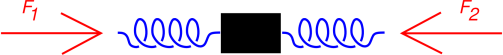
Note that there are two ways we can do work on an extended object. In figure 3, we have a mass (represented by the black rectangle) and two springs. We apply two forces, both directed inward. If the object yields a little in the inward direction, both forces do work. This increases the potential energy in the springs. This fits nicely into the well-known “PdV” category of work. This is not, however, the sort of work that is relevant to the “work/KE theorem” because no work is done against the center of mass of the object.
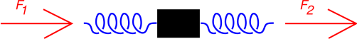
In figure 4 we have the same kind of object, with a mass and two springs. We apply two forces, both directed rightward. If the object moves a little in the rightward direction, both forces do work. This sort of work increases the kinetic energy of the object, in accordance with the “work/KE theorem”.
A parcel of fluid can be considered an extended object with many masses and many springs. When work is done on the parcel, there is a nontrivial question as to how much of the work goes into increasing the KE of the parcel and how much goes into increasing the PE of the parcel. As we shall see, Bernoulli’s principle is essentially the answer to this question.
This section is not finished. The equations are correct (as far as I can tell) but I haven’t finished fleshing out the explanations.
Suppose we have a parcel of air, flowing along a streamline in the usual way. We neglect viscosity and thermal conductivity. We consider what happens as it moves along a streamline. We assume the current state of the parcel is not very far away from some “reference” state indicated by subscript zero.
For present purposes, we will write equations that are accurate to first order. That is, we drop contributions that are second order in small quantities. For example, we do not care about the distinction between F0Δt and FΔt.
Also, in the interests of simplicity and clarity, we temporarily assume steady flow. The term describing unsteady flow can easily be added back in; see section 3.2. In this section we use the following symbols, in addition to the ones tabulated in equation 3:
| (22) |
We can calculate the change in pressure using the chain rule:
| (23) |
The average velocity is:
| (24) |
The net force acting on the parcel in the direction of motion is:
| (25) |
That allows us to calculate the impulse, i.e. the change in the momentum of the center of mass of the parcel:
| (26) |
Force and momentum are related by the second law of motion:
| (27) |
Combining the previous two equations and simplifying, we get
| (28) |
We can get rid of the deltas by comparing the “current” state to some “reference” state. Again we use a subscript zero to denote the reference state.
| (29) |
In particular, the average ⟨⋯⟩ is averaged over the path from the “reference” state to the current state.
We have used the fact that:
| (30) |
We remark that in the derivation leading up to equation 29, we did not attempt to calculate the entire energy or the entire change in energy of the parcel. Instead we calculated the impulse times the average velocity, which has dimensions of energy but is not numerically equal to the energy. There is more to physics than dimensional analysis, as discussed in section 4.6.
This derivation follows in the footsteps of the work/kinetic-energy theorem. We have calculated the change in the kinetic energy part of the energy. If we want to know the total energy, including the potential energy, we will need to do another calculation.
In any case, we have derived a simplified first-order expression describing the flow of a single parcel:
| (31) |
This is the most commonly-encountered form of “the” Bernoulli equation. It is not however the most robust; for careful work you should use equation 29 or equation 34.
The constant that appears on the RHS of equation 31 is called the stagnation pressure.
The following restrictions must be strictly observed:
This is the same as equation 29, keeping the term the represents the time-derivative of the pressure.
| (32) |
Next, we want to know what happens when our current state is not necessarily close to the “reference” state. For this we need some calculus, and we need the equation of state for the fluid, i.e. equation 8.
Using equation 29 and equation 8 we can continue the calculation as follows. We replace the finite deltas with derivatives. In the case where the pressure distibution is independent of time, we have:
| (33) |
Next, we integrate both sides. We make use of the fact that the mass of the parcel is constant (even while the pressure, volume, temperature, density, etc. are changing).
| (34) |
where K is some constant of integration.
Equation 34 is our main result. It is valid for any ΔP, large or small.
In subsonic situations, we are interested in pressure changes that are small compared to the “reference” pressure P0 (which we usually take to be the ambient pressure). That makes it useful to expand the LHS of equation 34 in a Taylor series. If we expand out to first order, we recover equation 29, as you can easily verify. It is more interesting to expand out to second order:
| (35) |
One reason why this equation is useful is that it tells you the range of validity of equation 29 and equation 31. Also it upholds the correspondence principle, by showing that the more general expression equation 34 reproduces the more familiar (but more restricted) results in the appropriate limit.
It is very common for people to state that equation 31 applies to a so-called “incompressible” fluid, since the equation treates ρ as a constant. Such a statement is complete nonsense. Equation 31 is routinely and correctly applied to air, which is quite compressible. The density definitely does change; indeed the percentage change in density is comparable to the percentage change in pressure. Indeed, all fluids – even liquids – are compressible to some degree. The validity of equation 31 does not depend on the fluid being incompressible. Not even approximately.
What’s even sillier is that to the extent that equation 31 is not exact, the correction term does not even involve the compressibility, as you can see from equation 35. The correction term depends on the adiabatic exponent γ, which is something else entirely. You cannot predict the compressibility based on γ or vice versa (except in the unphysical case where γ → ∞, which would imply constant volume i.e. zero compressibility).
Perhaps the key point is this: In situations where pilots would want to apply Bernoulli’s equation, it doesn’t matter (to a good approxmation) whether the air is compressible or not, provided the airspeed (v) is small compared to the speed of sound.
The explanation for this is quite simple: There is air pressure above the wing and below. In terms of absolute pressure, the two pressures are very nearly equal, so they give rise to equal-and-opposite forces.
If we are focused on lift and/or pressure drag, the only thing that matters is the difference in pressure. The total absolute pressure drops out of the force equations.
In contrast, the total density does directly matter. In equation 21, the difference in pressure appears on the LHS, but the total density appears on the RHS.
In the real world, in three dimensions, it is hard to imagine a fluid with an adiabatic exponent γ bigger than 1.667. However, very hypothetically, try to imagine a fluid where γ was very large. Then in the limit of γ → ∞ the volume of the parcel would have to be constant. In other words, the fluid would be incompressible. This can be seen in equation 8 or perhaps more directly in equation 17.
In this imaginary world, suppose we start with the second line in equation 10 and then take the limit γ → ∞. We can then treat V as a constant, and divide through by V. That leaves us with
| (36) |
which is essentially the same as equation 19.
It must be emphasized that the “derivation” leading up to equation 36 is nothing more than a mathematical fantasy, utterly devoid of any physical significance. The agreement between equation 36 and equation 19 is fortuitous, as far as I can tell.
We mention this because it is appallingly common to find books and web documents that say things like
Every part of that “explanation” is wrong. Although it’s true that equation 19 is only valid at low speeds, that’s simply because the equation is, by construction, a first-order approximation. This has got nothing to do with compressibility.
First of all, Bernoulli’s principle applies just fine to compressible fluids. Even the first-order approximation in equation 19 works fine for compressible fluids, which is a good thing, because there are no incompressible fluids. Furthermore, γ is not infinite. The γ for air is very nearly 7/5ths (i.e. 1.4), which is significantly less than infinity. The largest γ value of any fluid I know of is 5/3rds (approximately 1.6666) in the case of helium, and there theory suggests that γ can never be much larger than this for ordinary fluids.
Saying that «If the fluid had γ → ∞ it would be incompressible» is an absurd counterfactual statement, analogous to saying «if frogs had wings they wouldn’t have to jump». The fact is that frogs don’t have wings, and γ is nowhere near infinity.
It is also quite wrong to suggest that air is «more nearly incompressible» at low airspeeds. Air is obviously compressible. Neither the γ nor the compressibility is a function of airspeed. The γ value remains 1.4, right down to v=0.
While we are on this topic, note that γ is not even particularly closely related to compressibility.
It is a mystery how this nonsense about compressibility got started. One hypothesis is that it could be a case of multiple errors fortuitously canceling to produce a correct and useful result in equation 36. However, it is much more likely to be a Kiplingesque “just-so story” cooked up to explain a known result, cooked up by somebody who remembered the form of Bernoulli’s equation but didn’t remember how to derive it or even how to interpret it.
Some people have been “taught” that the first law of thermodynamics is:
| dE = −P dV + T dS (37) |
Alas, that is not the first law of anything. It’s not even true in general, as you can see by comparison with equation 2. Equation 37 cannot be valid unless we can express E as a function of the two variables V and S. In contrast, equation 2 is based on writing E as a function of four variables (V, S, h, and v).
The correct way to express the first law of thermodynamics is simply to express the local conservation of energy, as in equation 1.
Be careful not to oversimplify Bernoulli’s principle to the point where somebody says «high speed low pressure, low speed high pressure» or something like that. This gives grossly wrong answers when applied to any kind of pump or blower, or to a jet of fluid injected into an otherwise-undisturbed mass of fluid. You cannot use Bernoulli’s principle to compare one parcel “here” with another parcel “there” – unless you know a priori that the two parcels started out with the same head. The heads are flagrantly not the same in the typical grade-school demonstrations where somebody blows on a piece of paper. This is a very common mistake, but that does not make it any less of a mistake.
Also, you should be careful not to misinterpret simplified expression in equation 31. Remember:
More generally, we need to understand how to reconcile the simplified result equation 31 with the more robust result equation 34. In any situation where equation 31 applies, equation 34 applies also. This might seem to be a problem, because the two equations seem to say different things. One of them has a factor of γ/(γ−1) out front while the other doesn’t. Of course it’s not really a problem; the two equations are consistent, as demonstrated in section 3.4.
The key point is that the V in equation 34 is the real volume. It changes when the pressure changes. If/when you differentiate equation 34 to recover the first-order expression equation 31, you must take into account the variation in V.
For practical work, we should eliminate the V from equation 34 using the equation of state, as in equation 12. The latter looks more complicated, but it is in fact easier to use, because it depends on fewer variables.
Bernoulli’s equation is often “explained” as being an application of the principle of conservation of energy. That might seem plausible at the level of dimensional analysis, since in e.g. equation 31, ρ0 v2 is the kinetic energy per unit volume, and the pressure P has dimensions of energy per unit volume. Alas, this argument is not correct. There is more to physics than dimensional analysis. The pressure P is not equal to the actual energy per unit volume. Actually, for nonmoving air, the pressure is numerically equal to about 40% of the energy per unit volume.