Figure 1: Why Aliasing Must Happen
For reasons that will be explained below, I define my basic discrete Fourier transforms as follows:
| (1) |
(with an explicit factor of dt), while the corresponding inverse transformation is:
| (2) |
(with an explicit factor of df). Note the following:
The corresponding analog (non-discrete) Fourier transforms are:
| (3) |
| (4) |
We put the factor of 2π inside the integral, inside the exponential, where it belongs.
Suppose we have a vector Vin, representing a voltage waveform sampled at successive points in time. We wish to take the Fourier transform and then the inverse transform, which we denote rather abstractly as:
| (5) |
| (6) |
Let’s do an example. Suppose that our input data Vin is a Kronecker delta function in the time domain, that is:
| Vin = [1, 0, 0, ⋯⋯, 0] (7) |
The way the transform is defined in typical math books, and in typical software libraries, the normalization is such that Vf will be all ones:
| Vf = [1, 1, 1, ⋯⋯, 1] ☠ (8) |
This is not nice, but it is what you see in canned function libraries (such as fftw), in spreadsheet apps, and in scientific analysis programs (such as scilab or matlab).
The weird thing is that when the transform is defined this way, the inverse transform is defined to have a different normalization. As an example, if Vf is a Kronecker delta function in the frequency domain, and we take the inverse transform, Vout is not all ones; it is smaller by a factor of N, where N is the number of samples.
This leads to some pointed questions:
| ||Vin|| ≡ ||Vf|| ≡ ||Vout|| (9) |
so I guess we need to ask how to take the norm of such vectors.
Here are some answers. Reference 1 contains the scilab code to implement the solutions recommended here.
| dt = 1 millisecond (10) |
for a total of
| N = 2000 samples (11) |
Then the abscissas in the frequency domain will have a spacing of
| (12) |
| Vin = [1, 0, 0, 0, .... , 0] (13) |
then the forward transform should produce
| (14) |
which differs from the Vf in equation 8 by a nontrivial correction factor, namely a factor of dt.
| Vf = [1, 0, 0, 0, .... , 0] (15) |
then the inverse transform should be
| (16) |
which differs by two nontrivial correction factors from what you get from ordinary software packages. In particular, when using scilab, matlab, or the fftw library, the software automagically applies a factor of 1/N to the ordinates whenever it computes an inverse transform, so you need to undo that (by multiplying by a factor of N). Then you need to apply a further factor of df.
By the way, note that multiplying by (N df) is the same as dividing by dt. This means that if you perform a forward transform and an inverse transform, the correction factors discussed in this section drop out, and the corrected transforms really are inverses of each other.
In any case, in the time domain, the abscissa of the jth point is the time
| tj = j dt (17) |
Meanwhile, in the frequency domain, the abscissa of the kth point is the frequency
| fk = k df (18) |
which we can calculate via
| df = |
| (19) |
In equation 1 and equation 2, there are explicit factors of dt and df, respectively. These factors do not appear in the usual “textbook” definition of the transforms, but they have several advantages. For one thing, this makes the units come out right, in accordance with item 5. Secondly, this allows a high degree of symmetry between equation 1 and equation 2. In particular, I don’t need the ugly factor of 1/N that conventionally appears in the inverse transform.
(Don’t overlook the qualifiers “basic” and “discrete” that apply to this basic discrete Fourier transform. Equation 1 is not the most general notion of Fourier transform, as will be discussed in section 6.)
| (20) |
nor
| (21) |
Think about the Riemann integral: You don’t just sum up a bunch of ordinates; you need to weight each term in the sum by the measure of the corresponding abscissas.
Therefore the right answer is:
| (22) |
If you actually work out these quantities, using the Fourier transform as defined in equation 1, then the norm of the original data is equal to the norm of the transformed data, which means we are upholding Parseval’s theorem.
That is, the integral transforms are defined by equation 3 and equation 4.
Note that a big part of the trick is to think of frequencies (f) in circular measure (cycles per second, i.e. Hz) instead of frequencies (ω) in angular measure (radians per second).
Given that the input is sampled in steps of size dt, the output will always be periodic with a frequency equal to the sampling frequency, i.e. fS := 1/dt. The celebrated Nyquist frequency is half of that, i.e. fN := 0.5/dt. We have once again expressed f is in circular measure, and you can convert to radian measure if you want, in the obvious way, ω = 2πf.
The reason why aliasing occurs is obvious if you imagine that the input signal was built up from periodic waves to begin with. The signal component Vin = A G2π(f)t looks a whole lot like Vin = A G2π(f + fS)t or Vin = A G2π(f + k fS)t for any integer k, when sampled at intervals of dt. This works for any function G that is periodic with period 2π. The point is that the argument to G contains the term:
| (period) (k fS) t = (period) (k fS) i dt (23) |
for integers k and i. The factor of fS cancels the factor of dt, leaving only integer multiples of the period, so this term drops out.
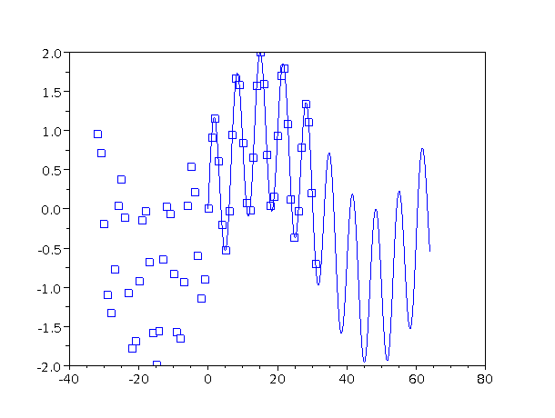
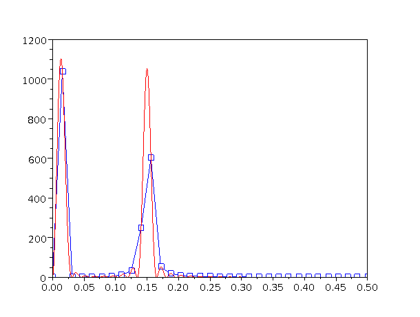
In figure 1 you can see how this works, i.e. why the output must be periodic in frequency space, whenever the input is sampled in the time domain.
We have a periodic function (shown in black) with period 1 (not 2π) and therefore frequency f=1. We sample it with sampling frequency fS=4. We also have a scaled version of the same function, scaled up in frequency by a factor of 5 in the time direction (shown in blue). (Multiplying the frequency by 5 is the same as adding 4 in this example. Recall that fS=4.) You can see that both functions go through the exact same sampling points (circled in red). So the scaled function is indistinguishable, sample-wise, from the original function. So if we perform Fourier analysis (or indeed any kind of frequency analysis) on sampled data, we will find that anything that happens at frequency f will happen again at frequency f ± fS and again at frequency f ± 2 fS, et cetera.
The scaled function may differ wildly from the original function in between sample points, but it always comes home at the sample points.
You cannot safely decide whether a signal is band-limited or not by looking at the sampled data! That would be like asking the drunkard whether he is drunk. For example, if I have a 100.01 Hz wave and sample it at 10.00 Hz, it will look like a beautiful 0.01 Hz signal. Ooops.
If you want to be sure that the original data is band-limited, rely on the physics, not on the math. That is, apply an analog filter to the signal, upstream of the digitizer. A real, physical, analog filter. If the filter passes negligible energy above the Nyquist frequency, then there will be negligible aliasing.
Standard good practice is to have the analog filter passband extend significantly above any frequency component you care about, so that you are not sensitive to details of the filter performance. Secondly it is standard good practice to sample at a sufficiently high rate that the Nyquist frequency is substantially above the passband of the filter. This means that you don’t need an analog filter with a fancy ultra-steep rolloff, while ensuring that no power gets through above the Nyquist frequency. When considered together, as in equation 24, these practices require that the sampling frequency be quite a bit higher than the highest frequency component of interest. This is called oversampling.
| (24) |
Oversampling by factors of 10 or more is common these days. That creates 10 times more sampled data than you might naïvely think was necessary. Some of that is necessary if you want any semblance of quality, and some of that can be removed by digital filtering after the data has been safely digitized. High-Q digital filters are much better behaved than high-Q analog filters.
This is somewhat a matter of taste, but I recommend choosing the sign of the imaginary unit (i) the way it appears in equation 1 and equation 3. This puts a minus sign in the expression defining the forward transform, and not in the inverse transform, which may not be the first thing you would have guessed. The advantage is that we want the signal
| Wf(t) = exp(+2 π i f t) (25) |
to be a wave with the frequency f. We do not want a minus sign in equation 25.
Note that the scilab program follows the convention I recommend. Some other software packages do not.
(If you are taking the transform of data that doesn’t have an imaginary part, you can’t tell the difference between positive frequency and negative frequency anyway, in which case it doesn’t much matter how you choose the sign of i.)
Non-experts sometimes want to have their cake and eat it too. That is, they want to have a plus sign in the exponential in equation 25 and a plus sign in the exponential in equation 1 also. This is not possible, because equation 1 has the form and function of an inner product. As discussed at e.g. reference 2, when complex numbers are involved an inner product must have the property that ⟨x,y⟩ = ⟨y,x⟩*, where the * denotes complex conjugate. There are many good reasons for this, including the fact that we want the inner product of something with itself to be a real number.
If you are doing anything involving Fourier transforms (including FFTs) you should make it a habit, every time you do a transform, to check that it upholds Parseval’s identity:
| (26) |
the factors of dt and df are important. The analog (non-discrete) version is:
| (27) |
If it fails that test, it means there’s something messed up with the normalization or the units or something. Remember that standard library functions know nothing about normalization; you have to do it yourself, prior to performing the Parseval check.
We now present several ways of obtaining a high-resolution Fourier transform. Section 6.1 presents the most advanced result, namely frequency-domain abscissas that are continuous, not discrete. Section 6.2 and section 6.3 present simple methods that are discrete, but with higher resolution due to finer spacing. Section 6.4 presents yet another method for obtaining the same result, in a way that is more mathematically sophisticated and more computationally efficient.
In all cases we are using the same raw time-domain data; we are improving the resolution of the frequency-domain results by using the data more cleverly.
Let’s talk about the following:
Sometimes people throw around the term “FFT” as if it were fully synonymous with Fourier transform. It is not.
FFT means Fast Fourier Transform, and is the name of a clever algorithm for performing a DFT efficiently. You could, if you wanted, perform the DFT using various less-efficient algorithms, and obtain a numerically-identical answer. In such a case it would still be a Fourier transform, just not an FFT.
The DFT has the interesting property that in general, if Vin consists of N complex values in the time domain, the transform produces N complex values in the frequency domain … and vice versa. In general, this number of samples is necessary and sufficient for the transform to be invertible. (There are some exceptions in cases where Vin and Vf have special symmetries.)
Let’s do an example. We consider the data shown in figure 2. The original data is the sum of two sine waves, as shown by the continuous curve in the figure. We sample the data at the 32 points indicated.
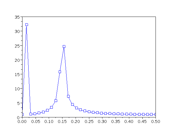
When we take the discrete Fourier transform, we obtain 32 points, namely the 17 points shown in figure 3, plus the mirror-image points at negative frequencies. The spacing between abscissas is df = 1/(32 seconds), i.e. 31.25 millihertz. Note that the ordinate is the magnitude of Vf, so we are not plotting the power spectrum, but rather the square root of the power spectrum.
We are now in position to discuss an important concept. Although, as previously mentioned, the N complex values are sufficient to make the transform mathematically invertible, invertibility is not the only consideration. The spectrum often has other uses, notably helping us to understand and communicate important facts about the signal. Plotting N points (as in figure 3) leaves out a lot of information, as we shall see in a moment.
We can define a more informative Fourier transform as follows: Start with equation 1 and eliminate k by substituting k → fk / df → fk N dt in accordance with equation 18 and equation 19. Then equation 1 becomes:
| (28) |
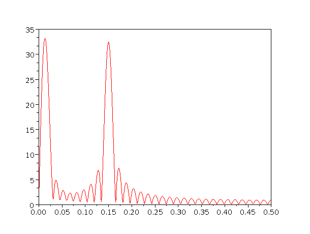
where the second line is a generalization, valid for all f whatsoever, not just integral multiples of df. This is illustrated in figure 4. You can see that figure 4 has vastly more detail than figure 3. This additional detail does not come from using more raw time-domain data; rather, it comes from using the existing data in more-informative ways. Both figures are based on the same 32-point time-series data.
You can see that equation 28 does not have (or need) any notion of df. This shouldn’t be surprising. The wave function Wf(t) as given by equation 25 is well defined for all times and for all frequencies. It is defined for all frequencies (fk) that happen to fit an integer number of cycles into the span of data (N dt) and for all other frequencies besides. It is defined for times (tj = j dt) that coincide with the data samples and for all other times besides. Equation 28 requires sampling the time variable to coincide with the data, but there is no requirement to sample the frequency variable.
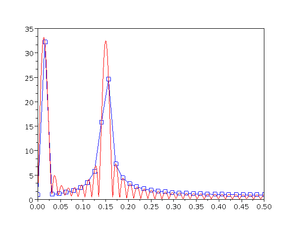
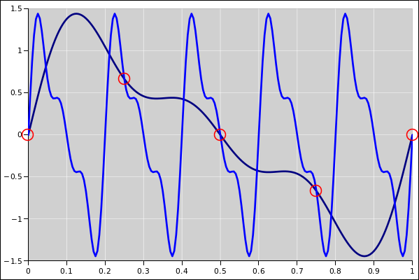
The relationship between figure 3 and figure 4 is easy to see if we overlay them, as in figure 5. The function Vf(⋯) defined by equation 1 is a subset of the function Vf(⋯) defined by equation 28. That is, Vf(f) is defined for all f, while Vf(f) is only defined for the isolated points f = k df. At the places where both functions are defined, they are equal.
Again you can see that the high-resolution transform has vastly more detail than the low-resolution transform. You may or may not be interested in this additional detail, depending on what problem you are trying to solve. Here are some common examples that illustrate the range of possibilities:
The limitations of the low-resolution transform look even more dramatic if we plot the power (rather than the magnitude), as in figure 6.
You can see that making a good spectrum analyzer is quite a bit trickier than simply making a call to the standard FFT subroutine. The following sections discuss various ways of increasing the resolution.
It is possible to increase the resolution of a Fourier transform while still maintaining some discreteness. This is less mathematically sophisticated than the fully continuous transformation, but may be more convenient for computation.
Here’s one way you could do this, if you wanted to rewrite the guts of the fourier-transform routines. This is not practical for the casual user, but it is worth discussing briefly, because it sheds some light on the fundamental issues. A more practical quick-and-dirty method is discussed in section 6.3 and a practical efficient method is discussed in section 6.4.
Suppose we want to have a large number of finely-spaced points in the frequency domain. Let Nt denote the number of raw data points in the time domain, and Nf denote the number of data points in the frequency domain. We want to have Nf ≫ Nt and therefore df = 1/(Nf dt) ≪ 1/(Nt dt). For some applications, such as visualizing the height, width, position, and symmetry of spectral features, we need to enhance the resolution by a factor (Nf/Nt) of at least 4, preferably 8 or even more.
We can generalize equation 1 by replacing each N that appears there by Nf or Nt as appropriate. That gives us:
| (29) |
which is more general than equation 1 (but less general than equation 28). The corresponding inverse transformation is:
| (30) |
Note that things are not quite as symmetric as you might expect, since Nf appears in the denominator inside the exponential in both the forward and inverse transform. That is related to the fact that we assume we are given some immutable time-domain data, and we are trying to increase the resolution in the frequency domain. The frequency spacing is
| df = |
| (31) |
This, plus the fact that there are Nf frequency-domain data points passed from the forward transform to the reverse transform, is sufficient to establish the orthornormality relationships that allow the inverse transform to properly undo the forward transform.
As another way to formulate the high-resolution Fourier transform, some people find it conceptually simpler to use equation 1, equation 2, and equation 19 as they stand, with the understanding that every N that appears there is Nf not Nt. That requires you to pad the time-domain data with Nf−Nt zeros, so that there are Nt “raw” time-domain points and a total of Nf “cooked” time-domain points. Such padding means it no longer matters whether the summation in equation 1 runs up to Nt−1 or Nf−1.
Reference 1 uses this trick, i.e. padding the input data with lots of zeros. This has the advantage of being easy to remember and easy to code. It is somewhat inelegant. It is less efficient than the method discussed in section 6.4, but not grossly inefficient, so unless you are doing huge numbers of transforms, it may not be worth your trouble to improve on it. (This assumes you are passing the data to a “fast” Fourier transform routing. In contrast, if you are using a brute-force un-fast Fourier transform, as in section 7, you will pay a high price for zero-padding.)
If you take the limit of large Nf in equation 29, it becomes effectively equivalent to equation 28. This reminds us of the key mathematical fact: The Fourier transform is well defined for any frequency whatsoever, even if you have a limited amount of time-domain data.
Some people question the validity of the generalization from equation 1 to equation 28, and also question the validity of padding the data with zeros. (After all, the real data isn’t zero, and anything involving fake data must be suspect.)
So, here is yet another method that obtains the same result. It should be pretty clear that this method is mathematically well-founded. Another advantage is that it is more computationally efficient. Indeed it is as efficient as it possibly could be.
The first ingredient in this method is the theorem that says multiplying two functions in the time-domain corresponds to a convolution in the frequency domain. The second ingredient is the observation that a frequency-shift can be considered a convolution, namely a convolution with a delta-function. The inverse Fourier transform is particularly simple; it is a trigonometric wavefunction of the form given by equation 25, where the f in that equation is the amount of the desired frequency-shift. So, the plan is to multiply the raw time-series data by a function of this form.
In the electronics and signal-processing field, multiplying by such a signal is called heterodyning. We will denote the amount of shift by fLO where “LO” stands for Local Oscillator.
You can verify that this works as advertised by doing some examples, perhaps using a spreadsheet as discussed in section 7.5.
If we heterodyne the raw data using a frequency shift that happens to be equal to df (i.e. the conventional “natural” spacing of points in the frequency domain), then it just shifts the frequency-domain data over one step. This doesn’t tell us anything new.
Things get much more interesting if we shift things by a fraction of df, let’s say a tenth of df for example, so that fLO = 0.1df. This shifts the frequency data by a tenth of a step. What does that mean? Well, recall that the basic discrete Fourier transform samples the continuous transform at the conventional points k df, as shown in figure 5. Sampling the heterodyned data at the conventional points is mathematically equivalent to sampling the un-heterodyned data at the unconventional points
| fk = kdf − fLO (32) |
which in this case is (k−0.1)df.
Note the minus sign in equation 32. The logic here is that when we multiply the raw data by a local-oscillator wave with positive frequency fLO, any feature that existed in the raw data lies at a higher frequency in the cooked data. Therefore if we apply a conventional FFT to the cooked data and see a feature at frequency kdf, we should associate that feature with a lower frequency kdf − fLO in the raw data. You can verify this numerically, as discussed in section 7.5.
Heterodyning gives us a highly quibble-resistant way of ascertaining what is going on “between” the conventional frequency-domain sampling points.
It is straightforward to prove (and/or verify numerically) that the methods suggested in section 6.2 and section 6.3 produce the exact same end results as the heterodyne method. This means that those methods were mathematically well founded all along, even if that wasn’t obvious until now.
Reference 3 is a spreadsheet that implements a Fourier transform, directly from the definition (equation 1) without calling any canned FFT library routines. This may help make the transforms less mysterious.
We start with N points of time-series data. N=8 should be enough for a start. (Later you can move on to N=32 if you are ambitious.) You can enter whatever ordinates you want in cells B12:C19 of the spreadsheet. The off-the-shelf version of the spreadsheet sets the input data to a wavefunction with frequency determined by the “fx” variable in cell C5. Feel free to change fx, or to completely replace the input data in cells B12:C19.
The time-domain cells are color-coded light blue. Similarly the graph of the time-domain data has a light blue background. In contrast, frequency-domain cells and the frequency-domain graph are color-coded light red.
Slightly to the right of time-series inputs, there is a rectangular table, N wide by N high, color-coded light green. It has time running vertically and frequency running horizontally.
Each cell of this table implements the complex exponential in equation 1. Since spreadsheets are not smart about complex numbers, we actually need two N×N tables, one for the real part and one for the imaginary part of the complex exponential … i.e. a cosine table and a sine table.
To implement the rest of the summation called for in equation 1, we use the sumproduct() function (rather than just the sum() function). The results are placed below the table, in cells F24:M25. These are color-coded light red, since they are frequency-domain data. There is also a graph of this data.
Note that there are N nontrivial frequency-domain points. That is, there is no “folding” or mirror-imaging. This is related to the fact that the input data had an imaginary part as well as a real part. (Without the imaginary part it would have been impossible to tell the difference between positive frequency and negative frequency, as you can easily verify by zeroing out the imaginary part of the input time-series data.) Actually I like to plot N+1 frequency-domain points, so that the plot better reflects the periodicity of the data.
We calculate the time-domain abscissas in cells A12:A19 based on the parameter dt in cell C4. We also calculate the frequency-domain abscissas in cells F23:M23.
We calculate the energy of the time-domain data and the energy of the frequency-domain data. These agree, as they should, in accordance with Parseval’s theorem. (The fact that we correctly calculated the abscissas is a big help when calculating the energy.)
It is amusing to change dt. Observe the effect on the abscissas, ordinates, and energies (in both the time domain and the frequency domain).
The inverse transform is implemented using the same technique. The complex exponential is in the yellow tables. The output of the inverse transform can be found in cells B33:C40. Below these cells is a check to confirm that the time-domain output agrees with the time-domain input.
If there are ND data points, there is absolutely nothing preventing you from implementing more than ND columns in the aforementioned tables. For example, you could easily double the number of columns (with a corresponding decrease in the column-to-column frequency spacing).
This produces higher resolution in the transform.
I implemented this in reference 4. There are still ND=8 time-domain data points, but there are now N=12 columns. The blue transformation tables are of size 8×12.
You can see that this is formally equivalent to padding the time-domain data with zeros and then using a 12×12 table. The spreadsheet omits the bottom four rows of the 12×12 since there is no point in doing a lot of multiplication by zero.
This also makes the point that Fourier transforms do not require the number of data points to be a power of two. Some canned FFT routines do require this, but the better ones do not. The FFT (if done right) is efficient for any highly-composite number, that is, any number that is the product of small primes. For example, if you have 37=2187 data points, it is more efficient to process that directly as 37, rather than rounding it up to 412=4096. And if you are using a non-fast Fourier transform, such as the direct brute-force Fourier transform in reference 4, then you can use any arbitrary number of points.
In the example in reference 4, since the frequency of the input data is 1/12th of a Hertz, fiddling with the resolution gives a better measure of the height of the peak in the frequency-domain data, since it allows the peak to fall on one of the calculated points.
More generally, though, increasing the resolution by a factor of 1.5 isn’t enough to accomplish much. If you are trying to measure the height and width of peaks, you need to oversample the frequency-domain data by at least a factor of 4, preferably a factor of 8 or more. If you want to see the advantages of higher resolution, look at figure 5 not reference 4 (or modify your copy of reference 4 to use vastly more columns).
What do you think will happen if we take the inverse of the high-resolution transform?
The spreadsheet in reference 4 contains an example of this. (You can think of this as the combination of section 7.2 with section 7.3.)
The spreadsheet in reference 5 implements heterodyning, of the sort discussed in section 6.4.
In the raw data, there is a peak at 0.1 Hz. This falls between steps in the conventional basic discrete Fourier transform, which has a stepsize of 0.125 Hz (i.e. 1/8th of a Hz, as expected, since there are 8 raw data points 1 second apart).
By using a LO frequency of 0.025 we can get a good look at the height of this peak. By using LO frequencies in the neighborhood of 0.025 we can learn about the width of this peak.
Feel free to change the LO frequency in cell G7 and see what happens. Values near 0 are interesting, and values near 0.025 are interesting.
In the frequency-domain plot (light red background), the red curve is the real part of Vf and the black curve is the imaginary part. The solid circles represent points calculated using heterodyning, while the circles with white centers represent points calculated without heterodyning, i.e. by applying the basic transform to the raw data. You can verify that the raw data and cooked data coincide if you set the LO frequency is zero.
This is just an introductory demonstration of some features of heterodyning. In a real application, you wouldn’t use a spreadsheet, and you would use the heterodyning trick repeatedly with many different LO frequencies (not just once as in this spreadsheet).
For large N, the brute-force method is not appropriate, but for small pedagogical examples it works just fine.
This is neither entirely the same nor entirely different from the way ordinary linear algebra uses column vectors and row vectors to represent contravariant and covariant vectors, i.e. pointy vectors and one-forms. One similarity is that if you scale up the intervals in the time-domain data, the intervals in the frequency-domain data get scaled down. One dissimilarity is that there is not (so far as I know) a meaningful contraction operation connecting the time-domain and frequency-domain data. (If this paragraph doesn’t mean anything to you, don’t worry about it.)
Fourier transforms, while useful, are not the be-all and end-all when it comes to analyzing periodic or quasi-periodic data.
You know the saying: «If your only tool is a hammer, everything starts to look like a nail.» People are so accustomed to using Fourier transforms that sometimes they think the Fourier transform “defines” what we mean by frequency content. It doesn’t.
As an example, consider the free-induction decay that is the raw data in a typical pulsed NMR (FT-NMR) experiment. It has a nice sinusoidal part, but that is convolved with a wicked sawtooth-shaped envelope due to the sudden rise and gradual decay. The Fourier transform, by its nature, responds to the envelope in ways that interfere with simple interpretation of the frequency-domain data. You can say that the sinusoidal component of the time-domain data is represented by the center of the peak, and the decay of the envelope is represented by the width of the peak … but what about the steep rise at the beginning of the pulse? That causes weird artifacts.
There are additional artifacts if the apparatus does not capture the entire tail of the decay.
Apodization is a kludge to camouflage the worst of the artifacts. Trying to understand apodization may not be worth the trouble.
Remember that a Fourier transform is basically a linear analysis, followed perhaps by some nonlinearity in the peak-finding step.
At some point, you may want to give up on the FT method entirely, and just do a full-blown nonlinear analysis. This takes a ton of computer power, and wasn’t possible in Fourier’s day (or even 20 years ago), but it is possible now.
In particular, consider the time-series data in figure 2. Would you say that there "is" power at the frequencies where there are wiggly feet in figure 4? The FT power spectrum says there “is” energy at these frequencies, but other types of analysis (such as curve-fitting a sum of sine waves to the raw data) would say no.
Similarly, what about the width of the peaks in figure 4? The Fourier transform method attributes some nonzero width to the peaks. However, curve-fitting could establish that there are really just two sine waves, one at frequency 0.0625 and the other at frequency 0.3, with virtually no uncertainty about these frequencies, and with no residuals i.e. no other frequency content.
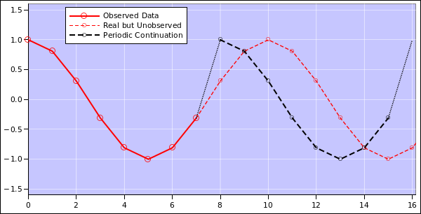
As another way to look at the same idea, the Fourier method is almost tantamount to assuming that the input data is periodic in the time domain, with period N dt. We can understand this with the help of figure 7.
In the figure,5 the red curve represents the real data. However, only the first 8 points (t=0 through t=7 inclusive) are actually observed, as shown by the solid dark red curve. Alas, the data has a frequency of 0.1 Hz, which is not commensurate with the 8-second span of the data. (A frequency of 0.125 Hz would have been commensurate.)
The Fourier transform method assumes the observed data will be periodically continued, as shown by the black curve. In this case there is a significant misfit between the unobserved real data and the periodic continuation of the observed data.
So in general, if your dataset doesn’t have a reasonable periodic continuation, or if it has a period incommensurate with N dt, then the whole Fourier approach is on shaky ground. Apodization may camouflage the worst of the problems, but you’ve still got problems. The real data in figure 7 is a perfectly nice sine wave, but the periodic continuation is not. This is a fundamentally unfixable problem, because the Fourier method blindly depends on the periodic continuation.
As another example, consider the so-called Fourier Transform Infra Red spectrometer (FTIR). The name FTIR is a misnomer in some ways. Non-experts commonly imagine that there is some sort of Fourier transform / inverse transform pair is involved, but there isn’t.
The crucial part of the machine is a Michelson interferometer, which performs an autocorrelation – not a Fourier transform. An autocorrelation is related to a Fourier transform via the Wiener-Khinchin theorem, but “related to” is not the same as “same as”.
In particular, the spectrum coming out of an FTIR machine shows a so-called “zero burst” which cannot be explained in terms of Fourier transforms, but is exactly what you would expect from an autocorrelation.
In the spirit of the correspondence principle, let’s examine the relationship between a discrete Fourier transform and a non-discrete Fourier transform. We start with a discrete transform and see what happens:
We can do another correspondence check, going in the opposite direction, i.e. starting with a continuous Fourier integral and converting it to a discrete sum. In a certain sense, that’s easy, because a sum is always a special case of an integral. From a measure-theory point of view, a sum is just an integral with a funny weighting function.
In particular, we can use the Dirac delta-function (δ) to apply unit weight to the places where we sample the waveform, and zero weight elsewhere. Examples include:
| (33) |
The first line of equation 33 is the defining property of the δ function. Once you buy that, the rest follows immediately by linearity. An integral is a linear operator.
If we plug this idea into the Fourier transform for continuous data (equation 3), we obtain the corresponding expression for sampled data:
| (34) |
which is the desired result. In the last line, we are free to write Vin(ti) in place of Vin(ti), because they are numerically equal. We can understand this relationship as follows: We can always express a function as a set of ordered pairs.1 As such, the function Vin() is is a subset of the function Vin(). That is, {(ti, Vin(ti))} ⊂ {(t, Vin(t))}. If we know Vin() it will tell us Vin() but not vice versa.
Note that even when the input consists of discrete samples, the result Vf() is defined for all frequencies.
The Vf on the LHS of equation 34 is not numerically equal to the Vf on the LHS of equation 3. The data being transformed is different, so we expect the results of the transform to be different.