|

| |
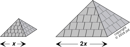
| Figure 1: Small-Scale Model Train | Figure 2: Large-Scale Model Train | |
There are many different scaling laws. At one extreme, there are simple scaling laws that are easy to learn, easy to use, and very useful in everyday life. Scaling laws can be and should be introduced at the elementary-school level, and then reinforced and extended every year through middle school, high school, and beyond. Scaling laws are central to physics. This has been true since Day One of modern science. Galileo presented several important scaling results in 1638 (reference 1 or reference 2).
This document is meant to be a tutorial, covering the simplest and most broadly useful scaling laws.
At the other extreme, there are more subtle scaling laws that are used to solve very deep and complicated problems at the frontiers of scientific research. The importance of scaling continues to the present day. There are dozens of references to “scaling” at the Nobel Prize site (reference 3).
Don’t let this scare you away. To repeat: this document is meant to be a tutorial, covering the simplest and most broadly useful scaling laws. You don’t need to be a Nobel laureate to get a lot of value from scaling laws.
You may be familiar with a simple form of scaling in connection with scale models, such as in figure 1 and figure 2. (The two figures are the same, except that one has a larger scale than the other.) The same word shows up in connection with small-scale and large-scale maps. For more about the terminology, see section 4.
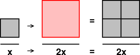
Perhaps the best known scaling law pertains to the relationship between length and area. In figure 3, when it comes to length, every length in the large square is twice as great as the corresponding length in the small square. When it comes to area, you can see that the area of the large square is not twice as great, but rather four times as great as the area of the small square.
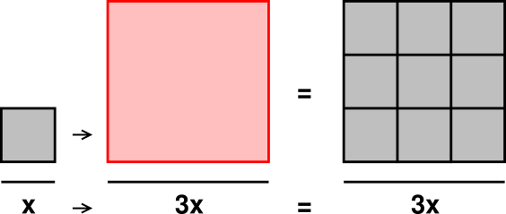
Now let’s see what happens if we scale up the lengths by a factor of 3 rather than 2. In figure 4, when it comes to length, every length in the large square is three times as great as the corresponding length in the small square. When it comes to area, the area of the large square is nine times as great as the area of the small square.
The general rule here is the so-called “square law”:
| (ratio of areas) = (ratio of lengths)2 (1) |
In words, the ratio of areas goes like the second power of the ratio of lengths. Equivalently, you can say that the ratio of areas goes like the square of the ratio of lengths.
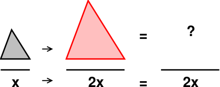
Continuing to examine the relationship between length and area, let’s see what happens with triangles. In figure 5, when it comes to length, every length in the large triangle is twice as great as the corresponding length in the small triangle. So the question is, how does the area of the large triangle compare to the area of the small triangle?
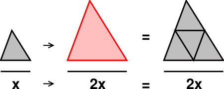
The right answer is that the area of the large triangle is four times the area of the small triangle, as you can see from figure 6.
So you can see that the “square law” in equation 1 is absolutely not limited to squares. In fact, squareness has got nothing to do with it.
The key idea here is that areas depend on width times height. So if the width is scaled up by a factor of K and the height is scaled up by a factor of K, the area necessarily gets scaled up by a factor of K2.
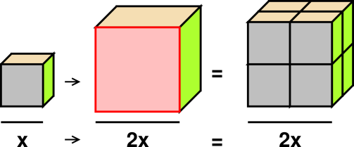
We can extend this idea into three dimensions, as shown in figure 7. When it comes to length, every length in the large cube is two times as great as the corresponding length in the small cube. When it comes to area, the surface area of the large cube is four times as great as the surface area of the small cube. When it comes to volume, the volume of the large cube is eight times as great as the volume of the small cube.
The volume goes up by a factor of eight because the cube is twice as wide and twice as deep and twice as tall. That’s three factors of two.
Meanwhile the surface area of the cube went up by a factor of four, not a factor of eight. That’s because on each face of the cube, the surface goes like width times height; the surface does not have any thickness. Each face of the cube is locally two dimensional, even though if you put all six faces together the total surface extends across three dimensions. Reconciling these facts requires a sophisticated notion of dimensionality. We say that the surface is intrinsically two-dimensional but is embedded in three dimensions.
The scaling laws for volume, area, and length can be expressed in terms of equations:
| (2) |
and if you want to get fancy, this can be expressed in one big equation
| (ratio of volumes)(1/3) = (ratio of areas)(1/2) = (ratio of lengths)1 (3) |
In equation 3, if a quantity has extent in N spatial dimensions, we take the Nth root.
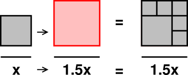
It is straightforward to scale things by factors that are not integers, as illustrated in figure 8. When it comes to length, every length in the large square is 1.5 times as great as the corresponding length in the original square. When it comes to area, the area of the large square is 2.25 times as great as the area of the original square.
You can confirm this graphically by counting squares on the far right of the diagram. Each of the tiny squares has 1/4th of the area of the original square. You can see that the large square has 9/4ths of the area of the original square.
You can understand the factor of 2.25 in several ways. One way is to take the ratio of lengths (1.5) and multiply it by itself using long multiplication. You don’t even need to do long multiplication if you remember that 15 squared is 225. Another way is to recognize 1.5 as 3/2, which you can square in your head to get 9/4, which reduces to 2.25. This corresponds to scaling up the lengths by a factor of 3 and then scaling down by a factor of 2.
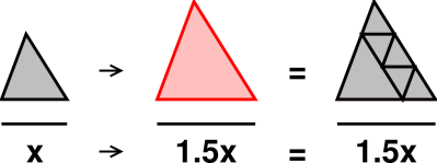
Of course the same thing works for triangles. When it comes to length, every length in the large triangle is 1.5 times as great as the corresponding length in the original triangle. When it comes to area, the area of the large triangle is 9/4ths as great as the area of the original triangle.
The scaling law for triangles is even more useful than the scaling law for squares, because it is easy to divide any polygon into triangles. By applying the scaling law to each of the triangles, you can easily prove that the scaling law must apply to any polygon.
Going one step further down that road, note that the area and perimeter of any ordinary (non-fractal) plane figure can be approximated as closely as you want by a polygon. For example, a circle is (for most purposes) well approximated by a many-sided regular polygon. In this way you can convince yourself that equation 1 applies to a very wide class of figures.
The same argument applies in three dimensions. First, convince yourself that equation 2 and equation 3 apply to any tetrahedron. Then note that any polyhedron can be divided into tetrahedra. Conclude that equation 2 and equation 3 apply to any polyhedron.
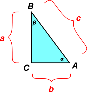
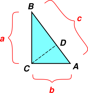
In principle, all of trigonometry is a collection of scaling laws, based on the idea of similar triangles. If you know triangle ABC has one right angle (as shown in figure 10) and you know one of the other angles (such as α), then you can infer the third angle. That triangle is similar to every other triangle with those three angles. All such triangles are related by a simple scale factor ... and length-ratios such as a/c, b/c, a/b are scale-invariant.
We can give names to these ratios:
- a/c is called sin(α),
- b/c is called cos(α),
- a/b is called tan(α),
and so on.
We start with the triangle ABC as shown in figure 11. We construct line CD perpendicular to AB.
Now we have three triangles: the lower triangle ACD which has hypotenuse b, the upper triangle CBD which has hypotenuse a, and the whole triangle ABC which has hypotenuse c. You can easily show1 that these are all similar to each other, so scaling arguments apply.
The upper triangle is a scaled-down copy of the whole triangle, with each length scaled by a factor of a/c. Similarly the lower triangle has each length scaled by a factor of b/c. The whole triangle, naturally, is scaled relative to itself by a factor of c/c = 1.
Area scales like length squared.
You can also see that the area of the whole triangle is exactly covered by the two smaller triangles, which means:
| (4) |
Equation 4 says that the area of the upper triangle plus the area of the lower triangle is equal to the area of the whole thing. The first expresses this in dimensionless terms, using the area of the whole triangle as the unit of area. The second line expresses the same thing using conventional dimensions of area.
The second line of equation 4 is the conventional way of stating the Pythagorean theorem. The first line is another way of expressing the same idea, and can also be interpreted as a thinly-disguised version of the trigonometric identity:
| sin2 + cos2 = 1 (5) |
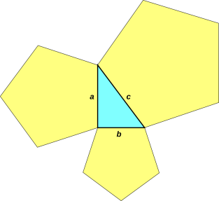
Here is another way to look at this proof: Whereas the traditional pictorial version of the theorem erects a square on the outside of each side of the triangle, we erect similar right triangles on each side of the original triangle.
The scaling idea is the same no matter what shape we attach to the edges of the triangle, so we could use pentagons, as shown in figure 12: the area of the a-pentagon plus the area of the b-pentagon is equal to the area of the c-pentagon. We can generalize this to any shape, so long as the three attached shapes are all similar to each other.
This can be considered a generalization relative to the usual statement of the theorem. This point was made by Euclid, 2300 years ago. See Proof #7 in reference 4, which is a collection of proofs of the Pythagorean theorem. The theorem can be applied to any shape, but the theorem is most easily proved using triangles, as in figure 11.
I really like the proof shown in figure 11, because it is easy and well-nigh unforgettable, it yields additional insights beyond what was required, and the method is transferable to a host of other problems (although I rate the “dot product“ proof slightly higher, based on the same criteria).
Tangential remark: If you’ve never seen the dot product proof, here it is: For any nonzero vectors a and b in an Euclidean vector space, let c = a+b. Then
| (6) |
Two nonzero vectors are called perpendicular if and only if their dot product vanishes. This is the definition of “perpendicular” in this sort of vector space.
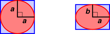
Consider the left half of figure 13. We see a circle inscribed in a square. The circle has area π a2 while the square has area 4 a2. That means that compared to the square, the circle has π/4ths of the area.
Now let us turn our attention to the right half of figure 13. We see an ellipse inscribed in a rectangle, in the ordinary symmetric way.
The right half of the figure is the same as the left half, except that the vertical lengths have been scaled by a factor of λ, such that b = λ a. (The horizontal lengths are unchanged.)
The question is, what about the area? If we had scaled all of the lengths (horizontal and vertical) by a factor of λ, then the area would be scaled by a factor of λ2 – but that is not the case here. In fact we scaled one length and not the other, so we pick up only one factor of λ. Therefore we expect the rectangle to have area λ 4 a2 i.e. 4 a b. This result can be verified by applying the elementary formula for the area of a rectangle.
As for the area of the ellipse, using the same scaling argument, we expect it to be scaled relative to the circle by one factor of λ. That is, we expect the area of the ellipse to be λ π a2, which is just π a b. This result can be verified if you happen to remember the formula for the area of an ellipse (π times the semi-major axis times the semi-minor axis).
Note that the dimensionless ratio π/4 is unchanged by the scaling as we go from left to right in figure 13. That means that compared to the square, the circle has π/4ths of the area ... and by the same token, compared to the rectangle, the ellipse has π/4ths of the area.
| = |
| = |
| (7) |
If you want an absolutely rigorous proof of this result, you can express the area in terms of an integral, and then do a change of variable. The resulting factor of b/a then pops out in front of the integral, since an integral is a linear operator. That means you don’t even need to evaluate the integral in order to obtain the scaling result.
A more intuitive explanation for why this works has two parts: First, there is an area-to-area scaling rule: We expect the area of one thing to scale like the first power of the area of another thing. So when we go from left to right in figure 13, we scale the area of the square by a factor of b/a, and also scale the area of the circle by a factor of b/a.
As a corollary, since we have pairs of areas, the ratio of areas is a dimensionless number (π/4ths for these particular pairs) and this dimensionless ratio scales like the zeroth power of the scale factor. That is, whenever a scale factor appears in a numerator in equation 7, it is canceled by an identical scale factor in the corresponding denominator.
This example illustrates that scaling arguments are more powerful than basic dimensional analysis. Since we have two lengths in the problem (a and b) and we are looking for an area, there are lots of expressions that have the correct dimensions; this includes ab, a2 + b2, (a+b)2, and various more-complicated possibilities.
Also: Reference 5 uses figure 13 as the starting point for a discussion of the relationship between memorizing things and rederiving things.
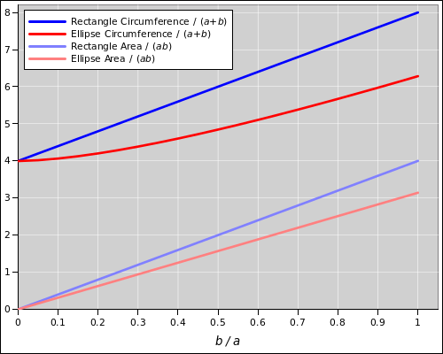
Now let’s consider the circumference of the ellipse. Beware that reasoning by analogy does not work in this case, but let’s give it a try, to see what goes wrong.
As discussed in section 1.7.1, the area of an ellipse is smaller than the area of the circumscribed rectangle by a factor of π/4. This is true no matter how round or how squashed the ellipse is.
Meanwhile, the circumference of an ellipse is smaller than the circumference of the circumscribed ellipse by a factor of π/4, provided the ellipse is perfectly circular.
If you checked only the three aforementioned cases, you might leap to the conclusion that the factor is always π/4, which would be unfortunate. It turns out that when the ellipse is squashed, its circumference is 100% of the circumference of the circumscribed rectangle. This is summarized in equation 8. The general case is graphed in figure 14.
| (8) | |||||||||||||||||||||||||||||||||||||||||||||||||||||||||||||||||||||||
The formula for the circumference of an ellipse is surprisingly complicated, as discussed in reference 6. There is no simple scaling law that applies here.
This is a reminder that scaling arguments have some serious limitations. See section 7.3.
Suppose we want to make a movie of an enormous pendulum clock, and we want the physics to look correct. The obvious way to do it would be to build a full-sized clock and film it using a normal camera.
However, there is another way to do it. We could build a scale-model clock, and then film it in slow motion. In other words, we modify both the length-scale and the time-scale. If we do this correctly, the result looks entirely natural. Specifically, the scale-factor applied to the time must be the square root of the scale-factor applied to the length, as mentioned in item 8.
Let us focus on the specific question of whether the behavior will look correct. To answer this question, at first glance it seems we need to know two things, namely the time-scale (t) and the length-scale (L). However, because there exists a scaling law, we really only need to know one thing, namely the ratio t/√L.
As a more extreme example, consider the question of whether the flow past a sphere will be turbulent. To answer this question, at first glance it seems we need to know four things, namely the speed (V), the size (L), the fluid density (ρ), and the viscosity (µ). However, because there exists a scaling law, we really only need to know one thing, namely the Reynolds number, i.e. the ratio ρVL/µ, as mentioned in item 32.
Any scaling law fits this pattern: It reduces the number of variables that you need to worry about. Actually, any law of nature fits this pattern, if you want it to. Usually the name “scaling law” is restricted to cases where the law involves some product of powers of the original variables.
The idea of replacing many variables by fewer variables has been rediscovered multiple times in various contexts, and has been given multiple different names. One way to describe it is to say that the correct physics occupies a subspace within the full parameter space. In the context of statistics, the same idea goes by the name sufficient statistic. In the context of critical-point physics, the same idea goes by the name of universality.
Scaling is not necessarily a mindless one-step process. Sometimes an equation that has useful scaling properties comes to you in a form where the scaling is not obvious. So you have to do some work to get the equations into a form where scaling laws can be derived and/or the number of variables can be reduced.
This commonly includes substituting a different set of variables. Sometimes the new variables are dimensionless groups (such as Mach number or Reynolds number) but sometimes not.
An example can be found in reference 7.
Part of the skill in making good scaling arguments involves using good terminology and avoiding bad terminology.
Here is some bad terminology: In figure 6, for example, it is dangerous to say that the big triangle is twice as large, or twice as big, or has twice the size of the small square. That’s because depending on the context, largeness and bigness and size could refer to the lengths involved, or could equally well refer to areas or volumes. Example: In a very practical sense, a two-liter bottle of water is “twice as big” as a one-liter bottle, even though its height and diameter are only 1.26 times as big.
This comes a shock to some people, and it is certainly inconvenient, but if you want to be careful you must avoid any unqualified statement about largeness, bigness, size, et cetera. If you mean length, say length. If you mean area, say area. And so forth. As an example, note that in section 4.2, we do not compare object A to object B; we compare the volume of A to the volume of B.
Here is some good terminology: People who are adept at making scaling arguments say things like this routinely:
The term “scale factor” is treacherous. Sometimes it refers to the ratio of lengths, but not always. On maps, it refers to the inverse ratio of lengths. That means that a large-scale map has a small scale factor (such as 50 miles to the inch), while a small-scale map has a large scale factor (such as 500 miles to the inch). This is a source of endless confusion among non-experts, and even experts get it wrong sometimes. I try to avoid the term “scale factor” whenever possible.
The phrase “... k times greater than ...” is so problematic that it deserves detailed discussion.
Consider the following scenario: VA denotes the volume of object A, while VB denotes the volume of object B. We are given that VA = 12 liters and VB = 36 liters.
The first three of the following statements are good terminology, but then things go to pot:
Discussion: statement 1, statement 2, and statement 3 describe VB in absolute terms as a multiple of VA. In contrast, statement 4 describes VB in relative terms, as an increment relative to the amount of VA we started with; the increment, not the whole amount of VB, is given as a multiple of VA. In statement 5, the word “greater” (or “more”) is a comparative adjective, which might have hinted that we are describing VB by means of a relative increment, but the word “factor” overrides this hint and makes it clear that we are describing VB in absolute (not relative) terms. This may not be entirely logical from a grammatical point of view, but the meaning of this expression is reasonably well established. We deprecate both statement 6 and statement 7, because it is hard to know which of them is correct. The word “times” suggests that VB is being described in absolute terms, while the comparative adjective “greater” suggests that VB is being described by means of a relative increment. I can’t say which interpretation is correct; some authors assume one interpretation, while others assume the other. I recommend avoiding both versions entirely, and using something like statement 1 or statement 4 instead.
A different problem crops up in statement 8. Does the statement mean that every dimension of B (length, width, and height) is bigger by a factor of 3, or does it only mean that the volume is bigger by a factor of 3? When you are scaling some property, you need to be specific about which property you are scaling.
In Euclidean geometry, objects that are the same except for scale and except for isometries (such as translation, rotation, and reflection) are said to be geometrically similar. (Beware: This conflicts with the non-technical use of “similar” to mean merely approximately alike.) Objects that are geometrically similar and have the same scale are said to be congruent.
The word “scale” in this context has the same meaning as in terms like scale model, and large-scale or small-scale maps. It is etymologically related to such things as the graduated scale on a burette. It is distantly related to the musical scale. It is unrelated to such things as the scales on a fish, or the scales used for weighing things.
The simplest forms of scaling are also known as proportional reasoning – but more generally, scaling laws go far beyond simple proportionality.
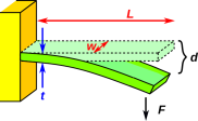
Stiffness is the inverse of compliance. The meaning of stiffness and compliance can be seen in figure 15. The left end of the beam is held fixed, while the right end is free to move.
When we apply a force F, the beam is deflected a distance d relative to its resting position. Then we say the stiffness (or spring constant) is k, where
| k = |
| (9) |
and the compliance is 1/k.
Now the interesting thing is that if the beam has length L, width w, and thickness t, the stiffness scales like w (which is unsurprising), and also scales like the cube of t/L.
| k ∝ w | ⎛ ⎜ ⎜ ⎝ |
| ⎞ ⎟ ⎟ ⎠ |
| (10) |
This cube law may comes as a surprise to some people. As discussed in section 6, breaking strength scales like cross-sectional area (in this case, width times thickness), and you might expect that stiffness would scale the same way, but it doesn’t.
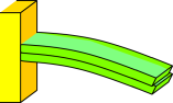
A beam that is twice as thick is vastly stiffer than two beams in parallel, as shown in figure 16.
Look what happens if you bend two beams that are not connected, just placed in parallel. The stiffness scales like the number of beams, i.e. like the total thickness. However, the free ends of the two beams don’t line up, as you can see if you look closely at figure 16.
In contrast, if you have a double-thickness beam – or a pair of beams glued together so that they can’t slide relative to each other – then the ends are forced to line up. That means when you bend it, the top half gets stretched and the bottom half gets compressed. This stretch and compression involves a lot of energy, and contributes greatly to the stiffness.
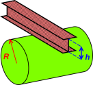
An I-beam is designed to cultivate this effect, as shown in figure 17. If you try to wrap an I-beam around a cylinder of radius R, the inner flange will try to follow a circle of diameter 2πR, while the outer flange will try to follow a circle of diameter 2π(R+h), where h is the height of the web. Since the two flanges started out the same length, and the web will keep the two flanges lined up, you can’t bend the I-beam without compressing the inner flange and stretching the outer flange. This makes an I-beam very much stiffer than a solid bar of comparable weight. See reference 8.
Breaking strength (unlike stiffness) scales simply like cross-sectional area.
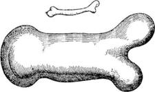
Following Galileo, let’s see what this implies about the bones of animals. The weight of the animal scales like linear size cubed. If we just scaled up the bones in proportion, the breaking strength would scale like linear size squared, which is not enough to keep up with the weight. Therefore the bones of a large animal must be not just thicker, but disproportionately thicker.
The thickness must scale like linear size to the three-halves power. Galileo published this result in 1638 (reference 1, page 170 of the National Edition). Figure 18 is a copy of his original drawing, showing a scaled-up picture of a small animal’s bone, compared to an actual large animal’s bone. (He doesn’t say exactly which animals he is comparing.)
Galileo also says (ibid)
I believe that a little dog might carry on his back two or three dogs of the same size, whereas I doubt if a horse could carry even one horse of his own size.
If something scales like xN, its derivative with respect to x will usually scale like X(N−1). (There is an exception for N=0.) Sometimes the notation suggests this (as in dF/dx), but sometimes it doesn’t (as in ∇F).
By the same token, if something scales like xN, its integral with respect to x will usually scale like X(N+1). (There is an exception for N=−1.)
For example, the electrostatic potential of a point charge falls off line 1/r. The electric field falls off like 1/r2. The field of an electric dipole falls off like 1/r3. See also item 42.
Similarly, the gravitational potential falls of like 1/r, the gravitational acceleration falls off like 1/r2, and the tide-producing stress falls off like 1/r3. See reference 9.
The moment of inertia about a given axis is given quite generally by I = ∫r2 dm. For constant mass m, the moment of inertia scales like r2 times m. On the other hand, for constant density, the mass scales like r3 and the moment of inertia scales like r5 times density.
Scaling arguments are more powerful that dimensional analysis. See reference 10. See also section 10.3 and section 1.7.2.
Dimensions are not the same as units. See reference 11. There is a special class of problems where the task is simply to convert the units, e.g. converting gallons to cubic inches. For these problems, there is a cut-and-dried algorithm — the factor label method — that works fine.
| There is also a class of problems that involve a simple proportionality with no fudge factors, for instance distance/time/rate problems, Ohm’s law problems, mass/volume/density problems, et cetera. For these problems, getting the units right pretty much guarantees a complete solution. | This stands in contrast to other problems where there is a nontrivial factor out front, perhaps a factor of 4π (as in item 2) or whatever. Dimensional analysis will never suss out the correct factor. |
When we say something scales, or is scalable, we mean we can change the scale of the thing and it still makes sense. For example, a triangle is scalable, because if we change the size it is still a perfectly fine triangle.
There exist plenty of things that are not scalable. As pointed out in section 6, an elephant is not just a scaled-up elephant-shrew. That means the animal as whole is not scalable. If you look at the skeleton of the shrew, you know what the “natural” size of the animal must be; if you tried to rescale it substantially, the result wouldn’t make sense. There is a natural size-scale for this animal.
Skeletal strength is not the only issue; the metabolism of any creature will generate heat in proportion to volume, while the ability to dissipate heat into the environment scales like surface area. This causes problems for large creatures (too much heat buildup) and for small creatures (too much heat loss). For details, see reference 12 and reference 13.
Another example of a failed scaling argument is given in section 1.7.3.
If something is scalable, the thing makes sense on many different size-scales; if something is not scalable, there is only one size-scale that makes sense for it.
Often when a complex system is not scalable, it is because of a conflict between various subsystems. In the case of animals, the weight scales one way, and the strength of the bones scales another way. Either weight or strength is scalable separately, but when we put them together we get a conflict.
Atoms are not scalable. The Bohr radius is a natural size-scale for atoms that is fixed by the fundamental physics. You can’t make a scaled-up hydrogen atom … unless you monkey with the fundamental physics, and nobody knows how to do that in practice. (The fundamental constants are called constants for a reason. That doesn’t prove they are constants, but it means you should think twice before assuming they are easily variable.)
When part of the system scales one way and part scales another way, we can often obtain useful scaling laws that work over some part of the domain, often a very large part. For example, as discussed in reference 10, we have a good scaling law for long-wavelength waves and another good scaling law for short-wavelength waves. Each of these laws is valid within its part of the domain; it is only in the crossover region that we see non-scalable behavior.
Many scaling laws work exceedingly well over a wide range of practical situations, but any scaling law applied to anything made of atoms must break down eventually, if you push it far enough, because atoms are not scalable.
Scaling laws are intimately connected to dimensional analysis; see reference 10 for an introductory discussion of the capabilities and limitations of dimensional analysis.
Always look for the scaling law. It might be obvious, or it might not. For example, if you can’t find a scaling law for some quantity X, maybe there is a nifty scaling law for (1−X). Keep looking.
Note that many scaling laws take the form of a power law, but not all; see item 35 in section 8.
The rationale here is simple: If you find a scaling law, it greatly increases your understanding of what is going on. Scaling laws are easy to use, and are very powerful.
Consider the relationship between scaling laws and detailed formal analysis. Neither is a substitute for the other; rather, they reinforce each other. The scaling law may sometimes tell you the answer you need, but even if it doesn’t, it suggests how to do the analysis. The analysis, in turn, may reveal additional scaling laws.
This is similar to the relationship between diagrams and formal analysis. Neither is a substitute for the other; rather, they reinforce each other.
Here are some interesting scaling laws. Some of them are self-evident, but some are not.
In particular, the surface area of a sphere scales like the square of the radius. The exact formula is:
| (11) |
Scaling and/or dimensional analyis and/or unit analysis will tell you the exponent on the RHS, but they won’t give you the factor of 4π out front.
Many people find this counterintuitive. They understand that the circumference of the ring will increase, and they understand that the outer diameter will expand outwards, but they erroneously expect that the inner diameter will move inwards. In fact the inner diameter increases along with all the other linear dimensions.
This is a fanciful example, but similar examples exist in the real world. Roads, bridges, and railroad tracks really do exhibit thermal expansion, and arrangements must be made to accommodate this. Also if you are welding something, you have to take thermal expansion into account. If it’s the right size when it’s hot, it won’t be when it cools off.
You need to scale the time by a factor of √N. That is, you shoot the explosion at a higher frame rate, so that when it is played back everything is seen in slow motion. In accordance with item 9, this means that each falling object falls through given (scaled) length in the appropriate amount of (scaled) time.
For simplicity, assume that the dominant cost is the energy required to lift the stone blocks into place, doing work against the gravitational field, starting from ground level. Assume the pyramid is a solid collection of blocks, not hollow inside.
It should come as no surprise that the fundamental constant є0 (the vacuum permittivity) has dimensions of farads per meter. This illustrates the connection between scaling laws and dimensional analysis.
This is an example of non-dimensional scaling. For details, see section 10.5.
Here’s a fancy example. Suppose we have a thermodynamic system with a certain set of extensive variables, such as volume (V), entropy (S), and the amount of each chemical component (Nν for all ν). Also suppose the energy can be expressed as a function of those variables.
It is more elegant to lump all the extensive variables into a vector X with components Xi for all i. (Energy is extensive, but not included in X.)
We introduce the general notion of homogeneous function as follows: If we have a function with the property:
| (12) |
then we say the function E is homogeneous of degree k. Here α is a scalar.
Applying this to thermo, we say the energy is a homogeneous function of the extensive variables, of degree k=1.
It is amusing to differentiate equation 12 with respect to α, and then set α equal to 1.
| (13) |
There are conventional names for the partial derivatives on the LHS: temperature, pressure, and chemical potentials. Note that these are intensive quantities (not extensive). Using these names, we get:
| (14) |
which is called Euler’s thermodynamic equation. It is a consequence of the fact that the extensive variables are extensive. It imposes a constraint, which means that not all of the variables are independent.
Note: Nothing is ever perfectly extensive. There are always boundary terms that don’t scale the same way as the bulk terms. However, for big-enough systems, the boundary terms can be neglected, and this scaling analysis is an excellent approximation.
If we take the exterior derivative of equation 14 we obtain:
| (15) |
which is called the Gibbs-Duhem equation. It is a vector equation (in contrast to equation 14, which is a scalar equation). It is another way of expressing the contraint that comes from the fact that the extensive variables are extensive.
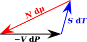
This has some remarkable consequences. For simplicity, suppose we have a system with only one chemical component. It may be tempting to visualize the system in terms of a thermodynamic state space where dT, dP, and dµ are orthogonal, or at least linearly independent. However, this is impossible. In fact dµ must lie within the two-dimensional state space spanned by dT and dP. We know this because a certain weighted sum has to add up to zero, as shown in figure 21.
The Gibbs-Duhem equation has many other practical applications.
In some cases, you already know a non-dimensional scaling law, and all you have to do is write it down and recognize it as a scaling law, as in section 10.5.
In other cases, we need to discover the non-dimensional scaling law. As we shall see, that involves two key steps:
Dimensional analysis will help you with step (a), but it cannot possibly help you with step (b). Sometimes people with a superficial understanding of dimensional analysis expect it to tell them everything they need to know. In fact, for all but the simplest problems, dimensional analysis is less than half the battle.
There are some fields such as fluid dynamics where you will never get past Square One unless you understand non-dimensional scaling.
As mentioned in item 20, the distance (s) to the apparent horizon scales roughly like the square root of your height (h) above the surface.
A more-detailed formula is:
where R is the radius of the earth. In words, equation 16b is the geometric mean of the eye-height and the diameter (not radius).
- Equation 16 neglects the effect of refraction in the atmosphere, which could be a substantial correction, on the order of 15%.
- Equation 16b assumes h≪R.
- Equation 16 approximates the surface as spherical. This is a terrible approximation if you are sitting at the bottom of a crater, but a good approximation over open water. (Even over water, the true radius varies with latitude, but this is only a fraction of a percent.)
This is a favorite introductory example of non-dimensional scaling. It shows that scaling laws are more general than dimensional analysis. Equation 16b is a nice scaling law that could not have been derived from dimensional analysis alone.
There are two physically-relevant lengths in the problem, namely the eye-height (h) and the radius of curvature (R) of the surface. Dimensional analysis can tell you that s ∝ hx R(1−x) = R (h/R)x, for some x … but it can’t tell you the value of the exponent x. Dimensional analysis doesn’t care whether x=0.5 or anything else, over a wide range. The existence of a physically-relevant dimensionless group (h/R) makes this a non-dimensional scaling problem, outside the reach of dimensional analysis.
Here’s an interactive online calculator, for finding the distance to the horizon. Input units can be feet, meters, km, or miles.
|
As foreshadowed in item 19, the mean free path (λ) of a particle in a gas of similar particles scales like the molar volume (V) of the gas divided by the scattering cross-section (σ) of the particle.
This example is interesting, because it demonstrates that scaling laws often depend on understanding the physics.
If you tried to find a scaling law for the mean free path by mindless application of dimensional analysis, you wouldn’t get far. There is a natural length in the problem, namely the average spacing between particles, which scales like the cube root of the molar volume. You might guess that the mean free path would scale the same way. Such a guess would pass the test of dimensional analysis, but it does not pass the test of real physics.
You may have noticed that there is another length in the problem, namely the square root of the cross section. That allows us to form the dimensionless quantity
| π1 = |
| (17) |
whereupon we could write the mean free path as
| (18) |
where the exponent a is (as yet) undetermined. Since π1 is dimensionless, dimensional analysis is powerless to tell us anything about the exponent a.
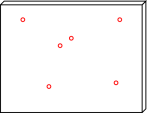
So let’s look at the physics. Let’s take a large region of the gas, roughly a cube of size D, and divide it into N thin layers. A view facing one such layer is shown in figure 22.
You can see that a particle incident on this layer would have a small probability of scattering against one of the particles in the layer. Call this probability p, with a lower-case p. The overall probability of passing through N such layers without scattering is
| (19) |
where P (with a capital P) denotes the probability that the particle will scatter somewhere in the N layers. Meanwhile, we also expect
| (20) |
which basically defines what we mean by the mean free path λ. Comparing these two equations, we expect p N to scale like D/λ.
We also expect p to scale like the number of particles in the layer, times the cross section of each particle. If we keep the molar volume constant, that means that p scales like σ D/N. Combining all the pieces, we find
| (21) |
That means we must have a=2 in equation 18, so the scaling law for the mean free path is
| (22) |
as advertised. This is a very simple, very useful result.
As another way of expressing the same result, we can approximate the average spacing between particles as
| (23) |
hence
| (24) |
We know that the density of a typical gas such as N2 or H2O at STP is about a thousand times less than the density of the corresponding liquid. That tells us that x is on the order of ten times larger than the size of the molecule. We can plug that into equation 24 to obtain an estimate that says the mean free path is probably about 100 times larger than the interparticle spacing at STP.
In contrast, in the interplanetary medium in the inner solar system, the interparticle spacing is on the order of 1 cm or slightly less. That means the mean free path is verrry long indeed.
Let’s consider the ultra-simple chemical reaction
| F2 ↔ 2F (25) |
and in particular let’s consider the equilibrium state in a vessel where that reaction is occurring in the gas phase. Let X denote the reaction coordinate, i.e. the degree to which the reaction has proceeded toward the right. Specifically, X=0 if we have 100% “reactants” (molecular F2), and X=1 if we have 100% “products” (monatomic F).
We choose conditions of temperature and molar volume such that X is initially small but nonzero. We hold the temperature constant, and increase the system volume V by moving a piston. We predict that increasing the volume by a factor of Q increases X by a factor of √Q.
Let’s work out the numbers for a simple scenario. We adopt the convention that in this context (a gas-phase reaction), square brackets [⋯] denote number density, i.e. the reciprocal of the molar volume. This is the convention used in introductory-level chemistry courses and in many advanced, practical applications. (If you are interested in activity rather than density, see below.)
Let’s consider the scenario shown in equation 26. We perform a step-by-step analysis, proceeding from state A via B to C. We arrange the initial state such that the F2 molecules have a number density of 2 moles per cubic meter. We arrange the temperature etc. such that the number density of unbound F atoms is less by a factor of 100. This initial condition is shown in column A in equation 26.
| (26) | ||||||||||||||||||||||||||||||||||||||||||||||||||||||||||||||||||||||||||||||||||||||||||||||||||||||||||||||||||||||||||||
As a first step, proceeding from state A to state B, we expand the system volume (V) by a factor of 2. We do this sufficiently quickly that we can temporarily ignore any chemical reactions; that is, we assume equation 25 takes place slowly whereas the expansion takes place quickly. The short-term result of the expansion is shown in column B in equation 26. Both number densities have gone down by a factor of two, while the reaction coordinate X remains unchanged. This is is an out-of-equilibrium situation.
As the final step, we allow the chemical reaction to come to equilibrium under the new conditions. The number density of unbound F atoms will increase. (This will deplete the density of F2 molecules, but only by a small percentage, which we ignore.)
The final state is shown in column C in equation 26. You can see that the total number of unbound F atoms is √2 larger than it was initially. (The density is lower, but the system volume is bigger, so all-in-all the number is bigger.) To say the same thing more precisely, the reaction coordinate X has increased by a factor of √2, as expected.
There are at least two simple theoretical arguments why this must be so. One is a subset of the argument that leads to the Saha equation (equation 28). The other considers the balance of reaction rates for the forward and reverse reactions. In any case, theoretically or otherwise, the inescapable fact is that the equilibrium value of the reaction coordinate X changes as we move the piston.
Another thing you can see is that the ratio in the bottom row is the same in both equilibrium situations. This leads us to define
| Kd := |
| (27) |
where the RHS is called the equilibrium ratio (aka equilibrium quotient) and where Kd is called the equilibrium “constant”.
We see that in equation 26, Kd has the same value in column C as it has in column A. That is, the equilibrium “constant” is constant under the conditions of this isothermal-expansion scenario. Alas, the equilibrium “constant” is not constant under other conditions. For starters, the equilibrium ratio – the RHS of equation 27 – is strongly dependent on temperature. So calling Kd the equilibrium “constant” is something of a misnomer.
There are good reasons why [F] appears squared in the numerator of the equilibrium ratio. There is a rule that says it must be squared because there are two units of F on the RHS of equation 25. The physical basis of this rule is connected to the fact that the recombination reaction F+F→F2 is a second-order process, in contrast to the disintegration reaction F2→F+F which is a first-order process. So you expect the rates for the two reactions to depend on density in different ways.
In equation 26, we would like to be able to predict the scaling based on the dimensions ... but we can’t. The scaling is highly nontrivial. We see that the equilibrium quotient has units of density, as do [F] and [F2]. Let’s consider the expansion and the expansion/reaction process separately:
There is no way you could have predicted this overall scaling behavior based on dimensional analysis.
This conflict between the dimensional analysis and the actual scaling behavior may look like a serious mistake, but it is not. It just shows the limitations of dimensional analysis. See section 10.3.2 for an explanation of how this comes about. As always, if the dimensions are telling you one thing and the scaling is telling you another, the scaling is incomparably more reliable because it is more closely connected to the physics. Dimensional analysis is only a hint as to how the scaling might go.
Here are the main points:
In equation 26, there are actually two volumes in the system. The obvious one is the system volume V. The less-obvious one is the quantum-statistical volume Λ3. Explaining all there is to know about Λ3 is beyond the scope of the introductory course. However, it exists and is crucial to understanding the scaling of Kd.
The bottom line is that if you scale the volume of the system, it changes more-or-less every density in the system, but it does not change Kd. Yes, Kd has dimensions of density, but it scales like the inverse of Λ3, not like the inverse of the system volume V. That’s why the equilibrium ratio actually remains reasonably constant when you scale the system volume at constant temperature.
Note: Sometimes you may be required to take the logarithm of Kd. The units of log(Kd) (as defined by equation 27) are nontrivial and must be carried additively (not multiplicatively), as discussed in reference 10.
If all you want is an introductory-level notion of what’s going on, stop here. The rest is beyond the scope of the introductory course.
Note: The example of a gas-phase reaction was chosen to keep things as simple as possible. However, the same ideas can be applied to reactants in solution. An ideal solution is closely analogous to an ideal gas. Concentration is almost synonymous with number density, in the appropriate units. In the gas-phase example we don’t need to worry about complications such as solvent-solute interactions.
We can begin to see what’s really going on if we look at the Saha equation. It is usually applied to the ionization of interstellar hydrogen, in which case it takes the form
| = |
| exp( |
| ) (28) |
where [np] is the number density of free protons, [ne] is the number density of free electrons, [nH] is the number density of neutral hydrogen atoms, and E is the hydrogen ionization energy, i.e. the Rydberg.
As usual, Λ denotes the thermal de Broglie length,
| (29) |
Comparing equation 28 with equation 27, we see that Kd has legitimate dimensions of inverse volume … but it does not scale like the inverse volume of the system. It scales like the inverse de Broglie length cubed. That means it depends on temperature and on immutable physical constants such as the mass of the electron.
We can use this to construct a dimensionless equation
| (30) |
where this K is dimensionless (unlike Kd). In fact this K is just equal to the relevant Boltzmann factor. Things could hardly get any nicer or simpler than this.
The trick is that on the LHS of the top line of equation 30, rather than using some arbitrary “unit” of volume when expressing densities per unit volume, we have used the physically-relevant quantum-statistical volume Λ3. (We slipped in the approximation that ΛH is very nearly equal to Λp.)
This (more-or-less) allows us to write
| K := |
| (31) |
where {⋯} denotes the dimensionless activity (in contrast to [⋯] which still denotes number density, as in equation 27). (See reference 18 for an introduction to the notion of activity.)
In equation 31, K is dimensionless and (as expected) scales like the zeroth power of system volume. However, this did not solve any of the fundamental problems. We saw in connection with equation 27 and equation 26 that we had three quantities, all with the same dimensions. Of these, one scaled V to the -1 power, one scaled like V to the -½ power, and one scaled like V to the 0 power. When we make things dimensionless, equation 31 still has three quantities, and one scales V to the -1 power, one scales like V to the -½ power, and one scales like V to the 0 power. There is obviously no way you can predict all three of these results using dimensional analysis. (The best you can do is play whack-a-mole, choosing dimensions so that one of the three scales the way its dimensions would suggest, while the other two conflict with their dimensions.)
We learned in high school algebra that it is OK to multiply both sides of an equation by the same thing. Therefore we can always convert equation 27 from dimensionful to dimensionless form by multiplying by some constant. This changes the dimensions of the equation, but it cannot possibly change the meaning! It’s just algebra. You should not imagine that equation 31 is in any way more correct or less correct than equation 27. They provably have exactly the same physical significance.
There is no escape from the fact that key elements of this problem are beyond the reach of dimensional analysis.
The key to understanding this is to note that there are two relevant volumes: the volume of the vessel, and the quantum-statistical volume Λ3. We can construct perfectly good scaling laws, provided we base them on honest-to-goodness physics, not mere dimensional analysis.
There is, alas, one huge fly in the ointment. In the context of chemistry, activity {⋯} is not conventionally defined using the quantum-statistical volume Λ3. Believe it or not, it is conventional to stick in some completely arbitrary ad-hoc volume instead, namely the molar volume of air at STP or something like that. That makes activity an illegitimate dimensionless quantity as discussed in reference 10 and reference 11. (You can make anything appear dimensionless using dirty tricks like that.) That trick also throws away the temperature dependence of Λ3, thereby disguising the temperature dependence of the equilibrium ratio. It’s awful.
Also beware that many authors denote activity by [⋯] as opposed to the {⋯} used here. This makes it difficult to tell at a glance whether density or activity is intended. Actually it is even worse than that, because you can find six separate definitions for [⋯], based on density, pressure, concentration, and the three corresponding activities.
Remark: The scaling properties of the equilibrium ratio provide a valuable lesson in the unity of statistical mechanics and thermodynamics. This is important because (believe it or not) there are some people who argue that the statistical definition of entropy (as discussed in reference 19) is somehow irrelevant to thermodynamics and to practical chemistry. Well, we see in this case stat mech is not just relevant, it is indispensable. Without it we would have no way to understand why activity is dimensionless yet scales like density. Classically there is only one relevant volume, namely the volume of the system. We need statistical mechanics to tell us about the other volume, namely Λ3. It is only after we know about both of those volumes that we have any chance of understanding the dimensions and the scaling.
Suppose a wave (aka ray) encounters the interface between one medium and another medium with a slightly different index of refraction. There will always2 be some reflection from such an interface. The amount of reflection depends on the angle, and on the change in index, in accordance with the Fresnel equations.
Let the relative change in index be called є. That is, n2 / n1 = 1 + є, for some small є. It may be helpful to think of є in terms of the logarithmic derivative: є = Δ(ln(index)).
You can show that at any particular angle, the amount of reflection scales like є squared. This is a famous result, worth remembering. Perhaps more importantly, you don’t need to remember it, because you can rederive it whenever you need it, just by looking at the structure of the Fresnel equations. Expand the RHS as a Taylor series in є. The zeroth-order term is zero, the first-order term is zero, and the second-order term is nonzero. This is an easy exercise in theoretical physics, involving little more than differentiating a polynomial. The coefficients of the polynomial are complicated functions of θ, but still it’s just a polynomial function of є. It’s even simpler as a function of n, and dn/dє = 1, so it comes to the same thing either way.
Depending on how you write the Fresnel equations, you may need to invoke Snell’s equation and/or the trig identity sin2 + cos2 = 1. I call that the “Pythagorean” trig identity, for obvious reasons.
We say that there is a universality property here. There is a universal curve for є2 Rp(є, θ), independent of є, when є is small.
We can immediately use this scaling law to understand that there should be no reflection from a gradual change in index. Divide the overall index change into N layers, with an index-change є on the order of 1/N at each boundary. The reflection per layer scales like 1/N2, so even if you add up all the layers, the overall reflection goes to zero in the large-N limit.
Suppose we randomly assign n items to d slots, and we care about the probability of a collision, i.e. two or more items in the same slot. For any given probability of collision, the number of items you can have scales like the square root of the number of slots.
A trivial example is the famous “birthday collision” question. Non-experts tend to guess that n should scale in proportion to d. That’s what simple notions of dimensional analysis would suggest, but it’s nowhere near correct.
Nontrivial examples crop up in lots of places, including in computer science (e.g. compiler construction) and in cryptography.
In more detail: Provided n ≪ d, the probability of collision is given (to a good approximation) by:
Note that this applies to the entire probability curve, not just the point where the probability equals 50%. This is an example of universality, as defined in section 2. That is, by invoking the scaling law, we can plot the entire curve as a function of the single variable n(n−1)/2d.
Equation 32b has the advantage of being strictly a power law, as is customary for scaling laws, whereas equation 32a has the advantage of being slightly more accurate when n is not very large.
You may have noticed that all the exponents in equation 2 are integers. These integers reflect the intrinsic dimensionality of the objects involved. Until fairly recently, most things were considered one-dimensional, two-dimensional, or three-dimensional … with nothing in between.
However, that’s not a hard-and-fast rule. There are some things that exhibit scaling exponents that are not integer, nor even rational numbers. Critical phenomena (as mentioned in item 40) are one example. Note that these are real, physical phenomena, not some perverse mathematical fantasy. Quasicrystals are another physical phenomenon with fractal properties.
The word “fractal” originally referred to fractional dimensionality. To make sense of that, you have to realize that it refers to Hausdorff dimension as opposed to the more familiar topological dimension.
According to the Hausdorff idea, we measure area – such as the area of a plane figure – according to how many disks of a given size it takes to cover the figure. Similarly we measure length – such as the length of the perimeter of the figure – according to how many disks it takes to cover the perimeter. We replace the idea of “scaling up the figure” with the idea of “using smaller disks”. Using smaller disks captures the same idea as “looking more closely” at the figure.
For ordinary (non-fractal) figures such as squares or triangles, the Hausdorff area scales like the square of the Hausdorff perimeter ... as expected.
In contrast, for fractals, if you look more closely you might see additional squiggly details on the perimeter, such that the perimeter grows more quickly than the square root of the area.
For more about fractals, see reference 20 and references therein.
The elementary type of scaling we are talking about today is part of a package of techniques for checking the work.
As always, some good advice is:
Check the units, check the dimensions, check the scaling more generally, check the symmetry, check that the vectors and scalars behave as they should, et cetera.
Following this advice may slightly increase the workload in the short run, but it greatly reduces the workload in the long run, especially when dealing with complex problems.
For example, in the neighborhood of equilibrium, to lowest order, the force had better be an odd function of x, and the energy had better be an even function. That is a symmetry check. It’s not exactly a scaling law, but it’s in the same spirit.
All such checks need to baked into the curriculum, like the oatmeal in oatmeal cookies; they can’t be sprinkled on afterwards. To say the same thing the other way, it does not make sense to have a National Scaling Day where everybody suddenly learns how to do scaling.
The scaling we are talking about here is not particularly tricky. If students are having a problem with it, the problem is almost guaranteed to not be a scaling problem per se. It is much more likely to be a symptom of a deeper problem, perhaps a poor grasp of basic algebra.
Some of the other things you can do with scaling – like conjuring up new equations out of thin air – involve serious industrial-strength wizardry. We can talk about that some other day.