So far we have discussed only a few basic ideas, but already we know enough to handle some interesting applications.
Let’s consider a Stirling engine. This is a type of heat engine; that is, it takes in energy and entropy via one side, dumps out waste energy and entropy via the other side, and performs useful work via a crankshaft.
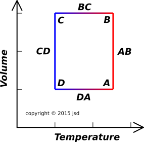
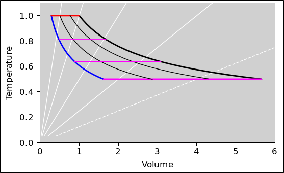
In operation, the Stirling engine goes through a cycle of four states {A, B, C, D} connected by four legs {AB, BC, CD, DA}. The Stirling cycle is rectangle in (T, V) space, as shown in figure 6.1.
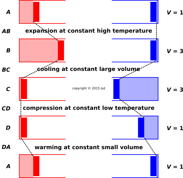
There are many ways of building a Stirling engine. The ones that are easy to build are not easy to analyze. (Actually all Stirling engines are infamously hard to analyze.) Let’s consider an idealized version. One way of carrying out the volume-changes called for in figure 6.1 is shown in figure 6.2. You can see that there are two cylinders: an always-hot cylinder at the left, and an always-cold cylinder at the right. Each cylinder is fitted with a piston. When we speak of “the” volume, we are referring to the combined volume in the two cylinders.
Let’s now examine the required temperature-changes. Figure 6.3 shows a more complete picture of the apparatus. In addition to the two cylinders, there is also a thin tube allowing the working fluid to flow from the hot side to the cold side and back again.
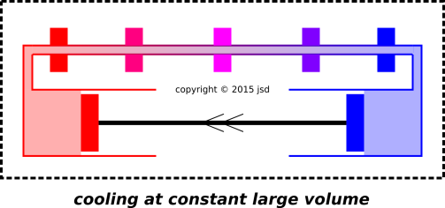
Figure 6.3 shows a snapshot taken during the cooling phase, i.e. the BC leg. The two pistons move together in lock-step, so the total volume of fluid remains constant. As the fluid flows through the tube, it encounters a series of heat exchangers. Each one is a little cooler than the next. At each point, the fluid is a little bit warmer than the local heat exchanger, so it gives up a little bit of energy and entropy. At each point the temperature difference is small, so the transfer is very nearly reversible. We idealize it as completely reversible.
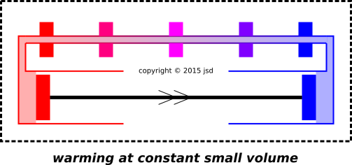
Figure 6.4 shows a snapshot taken during the warming phase, i.e. the DA leg. Once again, the two pistons move together in lock-step, so the total volume of fluid remains constant. The volume here is less than the volume during the cooling phase, so each piston moves less, but still they force all the volume to flow through the tube. (If you’re clever, you can arrange that the pistons move with less velocity during this leg, so that the overall time is the same for both the DA leg and the BC leg. That is, you can arrange that the flow rate in moles per second is the same, even though the flow rate in cubic meters per second is different. This gives the heat exchangers time to do their job.)
As the fluid flows through the tube, it encounters the same series of heat exchangers, in reverse order. At each point, the fluid is a little bit cooler than the local heat exchanger, so it picks up a little bit of energy and entropy. At each point the temperature difference is small, so the transfer is very nearly reversible. We idealize it as completely reversible.
The same number of moles of fluid underwent the same change of temperature, in the opposite direction, so the energy and entropy involved in the DA leg are equal-and-opposite to the energy and entropy involved in the BC leg. The molar heat capacity at constant volume is a constant, independent of density, for any ideal gas (or indeed any polytropic gas).
It must be emphasized that during the BC leg and also during the DA leg, no energy or entropy leaves the system. No energy or entropy crosses the dotted-line boundary shown in the diagram. The heat exchangers arrayed along the thin tube are strictly internal to the system. They do not require fuel or coolant from outside. They are like little cookie jars; you can put cookies and and take cookies out, but they do not produce or consume cookies. At the end of each cycle, they return to their original state.
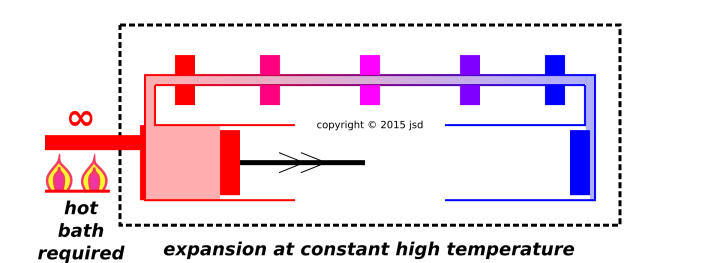
Figure 6.5 shows the expansion phase. The fluid is all on the hot side of the machine. The piston is retreating, so the fluid expands. If it were allowed to expand at constant entropy, it would cool, but we do not allow that. Instead we supply energy from an external source, to maintain the fluid at a constant temperature as it expands.
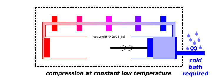
Figure 6.6 shows the compression phase. The fluid is all on the cold side of the machine. The cold piston is advancing, so the fluid is compressed into a smaller volume. If it were compressed at constant entropy, it would warm up, but we do not allow that. Instead we supply supply cooling from an external source, to maintain the fluid at a constant temperature during the compression.
It must be emphasized that the source that supplies energy and entropy on the left side of figure 6.5 is in a completely different category from the cookie jars attached to the flow tube. The source provides energy and entropy that flow across the boundary of the system. We imagine that the external high-side heat bath has an infinite heat capacity, so that we can extract energy and entropy from it without changing its temperature.
Similar words apply to the cooling system on the right side of figure 6.6. This is in a completely different category from the cookie jars, because energy and entropy are crossing the boundary of the system. We imagine that the low-side heat bath has an infinite heat capacity, so that we can dump energy and entropy into it without changing its temperature.
To summarize: Legs AB and CD are in one category (energy and entropy crossing the boundary, cumulatively, without end) while BC and DA are in another category (energy and entropy being rearranged interneally, with no net change from cycle to cycle).
The diagrams in this section do not show the crankshaft that delivers useful work to the outside. However we can easily enough figure out how much work is involved.
No work is performed on the BC leg or on the DA leg. The volume is the same before and after, so there is no PdV work. We are assuming an ideal engine, so the pressure on both sides is the same. The pressure changes during the BC leg (and during the DA leg), but at each instant the pressure at both ends of the machine is the same.
During the AB leg the volume increases by a certain amount, and then on the CD leg the volume decreases by the same amount. We know the fluid is hotter on the AB leg, so it has a higher pressure, so there is a net amount of PdV work done. For an ideal gas, it is easy to do the integral PdV. You don’t even need to assume a monatomic gas; a polyatomic ideal gas such as air is just as easy to handle. A factor of T comes out in front of the integral.
So, on a per-cycle basis, the energy that comes in on the left is proportional to Thot, while the energy that goes out on the right is proportional to Tcold.
We define the efficiency of a heat engine as
| (6.1) |
so for this particular heat engine, given all our idealizations, the efficiency is
| (6.2) |
Note that each hardware component in a Stirling engine sits at more-or-less steady temperature over time. The working fluid changes temperature significantly, but the hardware components do not. Increasing the thermal contact between the hardware and the fluid (at any given point) makes the engine work better. (On the other hand, we need to minimize thermal conduction between one cookie jar and the next, in the regenerator.)
A gas turbine engine (such as you find on a jet aircraft) is similar, insofar as the fluid changes temperature, while the hardware components do not, to any great extent. Also, the working fluid never comes in contact with hardware that is at a significantly different temperature. It is however in a different subcategory, in that improving the contact between the working fluid and the hardware will not make the engine work better.
This stands in contrast to a Carnot cycle, which depends on heating up and cooling down “the” cylinder that holds the working fluid. This is of course possible in theory, but it is troublesome in practice. It tends to reduce the power density and/or the efficiency of the engine. James Watt’s first steam engine suffered from this problem to a serious degree. It was only later that he figured out the advantages of having a separate condenser.
In a third category we have piston engines of the kind that you find in an ordinary automobile or lawn mower. They have the ugly property that the working fluid comes into contact with hardware at wildly dissimilar temperatures. This limits the efficiency, especially at low speeds. Making stronger contact between the working fluid and the cylinder walls would make the engine work worse. A similar temperature-mismatch problem occurs in the pistons of an external-combustion piston engines, such as piston-type steam engine, because the steam cools as it expands. (Of course a steam engine requires good thermal contact in the boiler and the condenser.)
As discussed in section 7.1, under mild assumptions we can write
| (6.3) |
We apply this to the heat baths that attach to the left and right side of our engine. We connect to the heat baths in such a way that we do not affect their pressure or volume, so we have simply:
| (6.4) |
Since for our engine, ΔE is proportional to temperature, we see that the amount of entropy we take in from the left is exactly the same as the amount of entropy we dump out on the right. (As always, it is assumed that no entropy flows out via the crankshaft.)
This property – entropy in equals entropy out – is the hallmark of a reversible engine. An ideal Stirling engine is reversible.
A heat engine operated in reverse serves as a heat pump. A household refrigerator is an example: It pumps energy and entropy from inside the refrigerator to outside. Other heat pumps are used to provide heat for buildings in the winter.
We now consider the class of all devices that
The claim is that all such engines are equally efficient.
The proof is stunningly simple and powerful: If you had two reversible heat engines with different efficiencies, you could hook them in parallel and create a perpetual motion machine!
As a corollary: We know the efficiency of all such devices (for any given pair of temperatures).
The proof is equally simple: Given that all devices that meet our three criteria are equally efficient, if you know the efficiency of one, you know them all. And we do know the efficiency of one, so we in fact we know them all. This is called the Carnot efficiency of a heat engine. It is:
| (6.5) |
As long as you are getting your energy from a heat bath, it is not possible to design an engine with greater efficiency than this, no matter how clever you are.
This is the glory of classical thermodynamics. Sadi Carnot figured this out long before there was a modern understanding of what energy is. The result depends on little more than the definition of temperature. In fact, the result can be turned around to serve as an operational definition of temperature: If you have an object at some known reference temperature, and another object at some unknown temperature, you can operate a reversible heat engine between the two, observe the efficiency, and deduce a value for the previously-unknown temperature.
Here’s another way of understanding the universal efficiency result. Imagine we have a heat engine that is reversible, but less efficient than we would expect based on equation 6.5. As a heat engine, it is less efficient, but as a heat pump it is more efficient! It is a too-good-to-be-true heat pump. As a heat pump, it takes in too much entropy on the cold side and ejects too little on the hot side. This violates the law of paraconservation of entropy (section 2.1).
It must be emphasized that the discussion in section 6.3 applies to heat engines and not otherwise. In particular, consider an electrochemical fuel cell. If it’s done right, the efficiency of such a thing vastly exceeds 1 − Tcold/Thot. That’s OK, because it’s not a heat engine. Even though it takes in fuel and puts out work, it is not a heat engine.
As an even more familiar example, consider a plain old electrochemical battery driving an electric motor. If it’s done right, the efficiency of such a thing vastly exceeds 1 − Tcold/Thot.
It is not worth the trouble to try to understand such things in terms of heat, or in terms of classical thermodynamics generally. I doubt it is even possible.
It is however straightforward to understand such things in terms of modern (post-1898) thermodynamics, i.e. statistical mechanics. Rather than getting bogged down trying to define “heat”, formalize everything in terms of energy and entropy instead. Entropy is defined in terms of probability, as a sum over states. In a battery, the state that stores the energy doesn’t even have a temperature, and it isn’t in equilibrium with your thermometer.
Let’s be clear: For a heat bath, its entropy is proportional to its energy, and the constant of proportionality is the inverse temperature. For a battery, that’s just not true. You can stick a lot of energy into a battery without changing its temperature.
We can derive a famous formula that places limits on the efficiency of any so-called heat-engine.
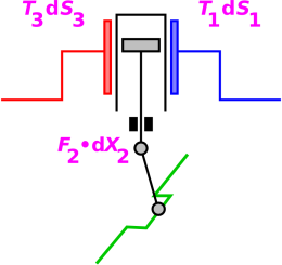
Figure 6.7 is a sketch of such an engine. The details don’t matter. The key concept is that the heat engine, by definition, has three connections, highlighted by magental labels in the figure.
Even though this is called a heat engine, trying to quantify the “heat” is a losing strategy. It is simpler and in every way better to quantify the energy and the entropy.
We could write the change in the energy content of the engine using equation 6.6, including all the terms on the RHS. However, as part of our definition of what we mean by heat engine, we require that only the terms shown in magenta are significant.
| (6.6) |
More specifically, we require that connection #3 be 100% thermal, connection #2 be 100% mechanical i.e. nonthermal, and connection #1 be 100% thermal. The engine is designed to segregate the thermal energy-transfers from the mechanical energy-transfers.
We have just constructed a theoretical model of an engine. This is a remarkbly good model for a wide range of real-world engines. However, it must be emphasized that it does not apply to all engines. In particular, it does not apply to batteries or to electrochemical fuel cells.
We must impose one more restriction: We require that the engine be able to operate in a cycle, such that at the end of the cycle, after doing something useful, all the internal parts of the engine return to their initial state. In particular, we require that the engine not have a “hollow leg” where it can hide unlimited amounts of entropy for unlimited amounts of time. This requirement makes sense, because if entropy could be hidden, it would defeat the spirit of the second law of thermodynamics.
Without loss of generality we assume that T2 ≥ T1. There is no loss of generality, because the engine is symmetrical. If necessary, just relabel the connections to make T2 ≥ T1. Relabeling is just a paperwork exercise, and doesn’t change the physics.
The engine starts by taking in a certain amount of energy via connection #3. We might hope to convert all of this heat-energy to useful work and ship it out via connection #2, but we can’t do that. The problem is that because connection #3 is a thermal connection, when we took in the energy, we also took in a bunch of entropy, and we need to get rid of that somehow. We can’t get rid of it through connection #2, so the only option is to get rid of it through connection #1.
For simplicity, we assume that T3 and T1 are constant throughout the cycle. We also make the rather mild assumption that T1 is greater than zero. Section 6.5.3 discusses ways to loosen these requirements.
Under these conditions, pushing entropy out through connection #1 costs energy. We call this the waste heat:
| (6.7) |
where the path Γ represents one cycle of operating the engine.
We can now use conservation of energy to calculate the mechanical work done by the engine:
where on the last line we have used that fact that the temperatures are unchanging to allow us to do the entropy-integrals. The deltas implicitly depend on the path Γ.
The second law tells us that over the course of a cycle, the entropy going out via connection #1 (−ΔS1) must be at least as much as the entropy coming in via connection #3 (+ΔS3). For a reversible engine, the two are equal, and we can write:
| (6.9) |
Where ΔS▸ is pronounced “delta S through” and denotes the amount of entropy that flows through the engine, in the course of one cycle. We define the efficiency as
| (6.10) |
Still assuming the temperatures are greater than zero, the denominator in this expression is just T3 ΔS3. Combining results, we obtain:
| (6.11) |
The maximum efficiency is obtained for a thermodynamically reversible engine, in which case
where equation 6.12b is the famous Carnot efficiency formula, applicable to a reversible heat engine. The meaning of the formula is perhaps easier to understand by looking at equation 6.12a or equation 6.11, wherein the second term in the numerator is just the waste heat, in accordance with equation 6.7.
Let us now consider an irreversible engine. Dissipation within the engine will create extra entropy, which will have to be pushed out via connection #1. This increases the waste heat, and decreases the efficiency η. In other words, equation 6.12b is the exact efficiency for a reversible heat engine, and an upper bound on the efficiency for any heat engine.
As a specific, important counterexample, a battery or an electrochemical fuel cell can have an efficiency enormously greater than what you would guess based on equation 6.12b ... even in situations where the chemicals used to run the fuel cell could have been used to run a heat engine instead.
The problem is, he’s asking the wrong question. Rather than asking how well he is doing relative to the Carnot efficiency, he should be asking how well he is doing relative to the best that could be done using the same amount of fuel.
Specifically, in this scenario, the guy next door is operating a similar engine, but at a higher temperature T3. This allows him to get more power out of his engine. His Carnot efficiency is 30% higher. His actual efficiency is only 20% higher, because there are some unfortunate parasitic losses. So this guy is not running as close to the Carnot limit as the previous guy. Still, this guy is doing better in every way that actually matters.
[This assumes that at least part of the goal is to minimize the amount of coal consumed (for a given amount of useful work), which makes sense given that coal is a non-renewable resource. Similarly part of the goal is to minimize the amount of CO2 dumped into the atmosphere. The competing engines are assumed to have comparable capital cost.]
Suppose you are trying to improve your engine. You are looking for inefficiencies. Let’s be clear: Carnot efficiency tells you one place to look ... but it is absolutely not the only place to look.
However, any heat engine still has a well-defined thermal efficiency, as defined by equation 6.10, even if the temperatures are changing in peculiar ways over the course of the cycle.
Furthermore, with some extra work, you can convince yourself that the integrals in equation 6.8b take the form of a ΔS times an average temperature. It’s a peculiar type of weighted average. This allows us to interpret the Carnot efficiency formula (equation 6.12b) in a more general, more flexible way.
By selecting a suitable set of the tiny Carnot cycles, you can approximate a wide class of reversible cycles. The efficiency can be calculated from the definition, equation 6.10, by summing the thermal and mechanical energy, summing over all the sub-cycles.
Because of the higher entropy, you might think the gas has less “available” energy (whatever that means). However, the hot gas contains more energy as well as more entropy, and it is easy to find situations where the hot gas is more useful as an energy-source, for instance if the gas is applied to connection #3 in a heat engine. Indeed, in order to increase efficiency in accordance with equation 6.12, engine designers are always looking for ways to make the hot section of the engine run hotter, as hot as possible consistent with reliability and longevity.
Of course, when we examine the cold side of the heat engine, i.e. connection #1, then the reverse is true: The colder the gas, the more valuable it is for producing useful work. This should make it clear that any notion of “available energy” cannot possibly be a function of state. You cannot look at a bottle of gas and determine how much of its energy is “available” – not without knowing a whole lot of additional information about the way in which the gas is to be used. This is discussed in more detail in section 1.7.3.
| (6.13) |
Both terms in the denominator here are positive; the second term involves a double negative.
We can understand this as follows: Whenever there are two thermal connections, one at a positive temperature and one at a negative temperature, the engine takes in energy via both thermal connections, and sends it all out via the mechanical connection. Therefore the efficiency is always exactly 100%, never more, never less.
Even if the engine is irreversible, such that −ΔS1 is greater than −ΔS3, the engine is still 100% efficient in its use of energy, because absolutely all of the energy that is thermally transferred in gets mechanically transferred out.
These conclusions are restricted to a model that assumes the engine has only three connections to the rest of the world. A more realistic engine model would allow for additional connections; see next item.
| (6.14) |