In this section we will illustrate the ideas using a scenario based on a heat engine. Specifically, it is a mathematical model of a reversible heat engine. For simplicity, we assume the working fluid of the engine is a nondegenerate ideal monatomic gas.
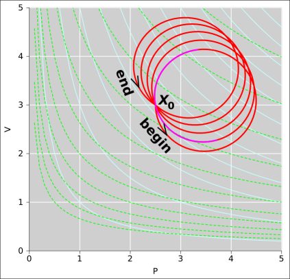
Figure 8.1 shows the thermodynamic state space for our engine. Such a plot is sometimes called the “indicator diagram” for the engine. The vertical white lines are contours of constant pressure. The horizontal white lines are contours of constant volume. The light-blue curves are contours of constant temperature ... and are also contours of constant energy (since the gas is ideal). The dashed light-green curves are contours of constant entropy. Given any arbitrary abstract point X in this space, we can find the values of all the state variables at that point, including the energy E(X), entropy S(X), pressure P(X), volume V(X), temperature T(X), et cetera. The spreadsheet used to prepare the figures in this section is cited in reference 22.
That’s nice as far as it goes, but it’s not the whole story. It is also useful to consider the path (Γ) shown in red in the (P,V) diagram. We will keep track of what happens as a function of arc length (θ) along this path ... not just as a function of state. We note that the path can be broken down into five approximately circular cycles. In this simple case, we choose units of arc length so that each cycle is one unit. Each cycle begins and ends at the point X0, which has coordinates (P,V) = (2.5,3) in figure 8.1.
Let’s use X to represent an arbitrary, abstract point in state space, and use XΓ(θ) to represent a point along the specified path. For simplicity, we write X0 := XΓ(0).
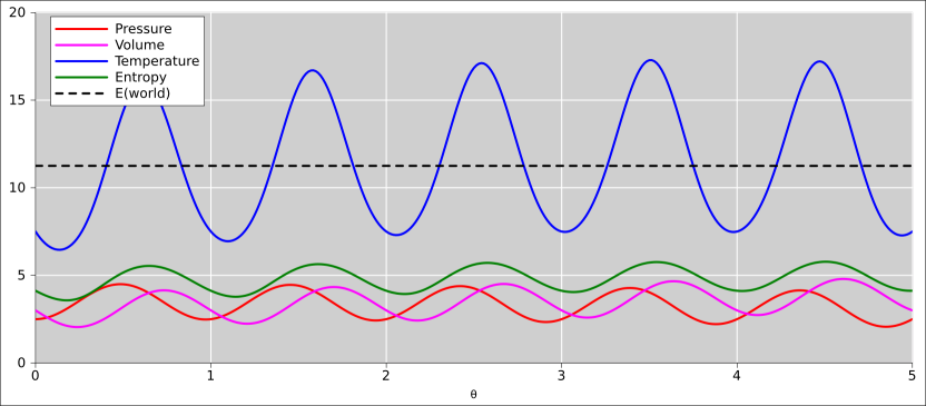
In figure 8.2, we plot several interesting thermodynamic quantities as a function of arc length. Whenever θ is an integer, the path crosses through the point X0. As a consequence, each of the variables returns exactly to its original value each time θ completes a cycle, as you can see in figure 8.2. There have to be definite, reproducible values at the point X0, since we are talking about functions of state.
In the spreadsheet used to create this figure, the path is chosen to be more-or-less arbitrary function of θ, chosen to give us a nice-looking shape in figure 8.1. The path tells us P and V as functions of θ. Temperature then is calculated as a function of P and V using the ideal gas law, equation 26.40. Entropy is calculated as a function of V and T using the Sackur-Tetrode law, equation 26.17. The order in which things are calculated is a purely tactical decision. Please do not get the idea that any of these state variables are “natural” variables or “independent” variables.
As discussed in section 7.4, as a corollary of the way we defined temperature and pressure, we obtain equation 7.8, which is reproduced here:
| (8.1) |
Each of the five variables occuring in equation 8.1 is naturally and quite correctly interpreted as a property of the interior of the engine. For example, S is the entropy in the interior of the engine, i.e. the entropy of the working fluid. However, in the scenario we are considering, the two terms on the RHS can be re-interpreted as boundary terms, as follows:
This re-interpretation is not valid in general, especially if there is any dissipation involved, as discussed in section 8.6. However, if/when we do accept this re-interpretation, equation 8.1 becomes a statement of conservation of energy. The LHS is the change in energy within the engine, and the RHS expresses the mechanical and thermal transfer of energy across the boundary.
Whether or not we re-interpret anything, equation 8.1 is a vector equation, valid point-by-point in state space, independent of path. We can integrate it along any path we like, including our chosen path Γ.
| (8.2) |
As always, “check your work” is good advice. It is an essential part of critical thinking. In this spirit, the spreadsheet carries out the integrals indicated in equation 8.2. The LHS is trivial; it’s just E, independent of path, and can be calculated exactly. The spreadsheet cannot evaluate integrals on the RHS exactly, but instead approximates each integral by a sum, using a finite stepsize. Rearranging, we get
| (8.3) |
This quantity on the LHS shown by the black dashed line in figure 8.2. It is constant to better than one part per thousand. This is a nice sensitive check on the accuracy of our numerical integration. It also tells us that our derivation of the ideal gas law and the Sackur-Tetrode law are consistent with our definitions of temperature and pressure.
If we accept the aforementioned re-interpretation, equation 8.3 tells us that our model system conserves energy. It accounts for the energy within the engine plus the energy transferred across the boundary.
Let’s give names to the two integrals on the RHS of equation 8.2. We define the work done by the engine to be:
| (8.4) |
where the integral runs over all θ′ on the path Γ, starting at θ′ = 0 and ending at θ′ = θ. We call WΓ the work done by the engine along the path Γ. This terminology is consistent with ordinary, customary notions of work.
We also define the heat absorbed by the engine to be:
| (8.5) |
For present purposes, we call this the heat absorbed by the engine along the specified path. This is consistent with “some” commonly-encountered defintions of heat.1
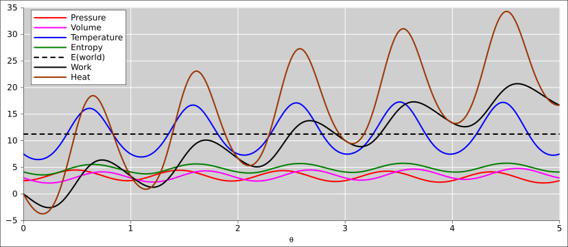
Figure 8.3 includes all the curves from figure 8.2 plus heat (as shown by the brown curve) and work (as shown by the black curve).
It should be clear in figure 8.3 that the black and brown curves are quite unlike the other curves. Specifically, they are not functions of state. They are functions of the arc length θ along the path γ, but they are not functions of the thermodynamic state X. Every time the path returns to the point X0 in state space, WΓ(θ) takes on a different value, different from what it was on the previous cycle. Similarly QΓ(θ) takes on a different value. You can see this in the figure, especially at places where θ takes on integer values. The state of the engine is the same at each of these places, but the heat and work are different.
Heat and work are plotted in figure 8.3, but there is no hope of plotting them on a (P,V) diagram such as figure 8.1.
Suppose we continue the operation of this heat engine for more cycles, keeping the cycles always in the vicinity of X0.
| The state variables such as P, V, T, et cetera will remain bounded, returning to their initial values every time the path Γ crosses the initial point X0. | The WΓ(θ) and QΓ(θ) curves will continue marching off to the northeast, without bound. |
| At any point X in state space, if you know X you know the associated values of the state functions, and the state functions don’t care how you got to X. | At any point X in state space, even if X is somewhere on the path Γ, knowing X is not sufficient to determine out-of-state functions such as QΓ(θ), WΓ(θ), or θ itself. The out-of-state functions very much depend on how you got to X. |
Suppose you start with T dS and you want to integrate it. There are at least three possibilities:
Please keep in mind that in modern thermodynamics, we define entropy in terms of the probability of the microstates, as discussed in connection with equation 2.2. However, back in pre-modern times, before 1898, people had no understanding of microstates. Quite remarkably, they were able to calculate the entropy anyway, in simple situations, using the following recipe:
The interesting thing is that even though this recipe depends explicitly on a particular path Γ, the result is path-independent. The result gives you S as a function of state (plus or minus some constant of integration) – independent of path.
Back in pre-modern times, people not only used this recipe to calculate the entropy, they used it to define entropy. It is not a very convenient definition. It is especially inconvenient in situations where dissipation must be taken into account. That’s partly because it becomes less than obvious how to define and/or measure QΓ.
In our scenario, we choose to operate the heat engine such a way that it moves reversibly along the path Γ in figure 8.1. Every step along the path is done reversibly. There is no law of physics that requires this, but we can make it so (to a good approximation) by suitable engineering.
We can also treat each of the five cycles as a separate path. If we do that, it becomes clear that there are infinitely many paths going through the point X0. More generally, the same can be said of any other point in state space: there are infinitely many paths going through that point. As a corollary, given any two points on an indicator diagram, there are infintely many paths from one to the other. Even if we restrict attention to reversible operations, there are still infinitely many paths from one point to the other.
As a separate matter, we assert that any path through the state-space of the engine can be followed reversibly (to a good approximation) or irreversibly. There is no way of looking at a diagram such as figure 8.1 and deciding whether a path is reversible or not. Reversibility depends on variables that are not shown in the diagram. Specifically, when some step along the path is associated with a change in system entropy, the step is either reversible or not, depending on what happens outside the system. If there is an equal-and-opposite change in the entropy of the surroundings, the step is reversible, and not otherwise.
I mention this because sometimes people who ought to know better speak of “the” reversible path between two points on a (P,V) diagram. This is wrong at least twice over.
As we shall see, state functions are more elegant than out-of-state functions. They are vastly easier to work with. Usually, anything that can be expressed in terms of state functions should be.
However, out-of-state functions remain importance. The entire raison d’être of a heat engine is to convert heat into work, so it’s nice to have a good way to quantify what we mean by “heat” and “work”.
An electric power company provides each customer with a watt-hour meter, which measures the electrical work done. The customer’s bill largely depends on the amount of work done, so this is an example of an out-of-state function with tremendous economic significance.
Also note that in pre-modern thermodynamics, “heat” was super-important, because it was part of the recipe for defining entropy, as discussed in section 8.1.3.
In cramped thermodynamics, heat content is a state function. You can heat up a bottle of milk and let it cool down, in such a way that the energy depends on the temperature and the heat capacity, and that’s all there is to it.
However, in uncramped thermodynamics, there is no such thing as heat content. You can define QΓ as a function of arc length along a specified path, but it is not a state function and it cannot be made into a state function.
More-or-less everybody who studies thermodynamics gets to the point where they try to invent a heat-like quantity that is a function of state, but they never succeed. For more on this, see section 8.2 and chapter 17.
If you ever have something that looks like “heat” and you want to differentiate it, refer back to the definition in equation 8.5 and write the derivative as T dS. That is elegant, because as discussed in section 8.2 and elsewhere, T is a state function S is a state function, dS is a state function, and the product T dS is a state function. This stands in contrast to QΓ which is not a state function, and dQ which does not even exist.
It is possible to differentiate QΓ if you are very very careful. It is almost never worth the trouble – because you are better off with T dS – but it can be done. As a corollary of equation 8.1, equation 8.4, and equation 8.5, we can write:
| (8.6) |
which is of course shorthand for
| (8.7) |
Whereas equation 8.1 is a vector equation involving gradient vectors, equation 8.6 is a scalar equation involving total derivatives with respect to θ. It can be understood as a projection of equation 8.1, obtained by projecting the gradient vectors onto the direction specified by the path Γ.
On the LHS of equation 8.6, we might be able to consider the energy E to be a function of state, especially if we we can write as E(X), which does not depend on the path Γ. However, if we write it as E(XΓ), the energy depends indirectly on the path. In particular, the derivative on the LHS of equation 8.6 very much depends on the path. Considered as a derivative in state space, it is a directional derivative, in the direction specified by the path.
Here is where non-experts go off the rails: In equation 8.6, it is tempting (but wrong) to “simplify” the equation by dropping the “dθ” that appears in every term. Similarly it is tempting (but wrong) to “simplify” the equation by dropping the Γ that appears in every term. The fact of the matter is that these are directional derivatives, and the direction matters a great deal. If you leave out the direction-specifiers, the derivatives simply do not exist.
Sometimes people who are trying to write equation 8.6 instead write something like:
| (8.8) |
which is deplorable.
Using the language of differential forms, the situation can be understood as follows:
where in the last four items, we have to say “in general” because exceptions can occur in peculiar situations, mainly cramped situations where it is not possible to construct a heat engine. Such situations are very unlike the general case, and not worth much discussion beyond what was said in conjunction with equation 7.37. When we say something is a state-function we mean it is a function of the thermodynamic state. The last two items follow immediately from the definition of grady versus ungrady.
Beware that in one dimension, ΔS is rather similar to dS. However, that’s not true in higher dimensions ... and uncramped thermodynamics is intrinsically multi-dimensional. If you have experience in one dimension, do not let it mislead you. Recognize the fact that ΔS is a scalar, whereas dS is a vector.
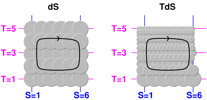
Figure 8.4 shows the difference between a grady one-form and an ungrady one-form.
| As you can see in on the left side of the figure, the quantity dS is grady. If you integrate clockwise around the loop as shown, the net number of upward steps is zero. This is related to the fact that we can assign an unambiguous height (S) to each point in (T,S) space. | In contrast, as you can see on the right side of the diagram, the quantity TdS is not grady. If you integrate clockwise around the loop as shown, there are considerably more upward steps than downward steps. There is no hope of assigning a height “Q” to points in (T,S) space. |
Some additional diagrams showing the relationship between certain grady and ungrady one-forms, see section 15.1.2. For details on the properties of one-forms in general, see reference 4 and perhaps reference 23.
Be warned that in the mathematical literature, what we are calling ungrady one-forms are called “inexact” one-forms. The two terms are entirely synonymous. A one-form is called “exact” if and only if it is the gradient of something. We avoid the terms “exact” and “inexact” because they are too easily misunderstood. In particular, in this context,
- exact is not even remotely the same as accurate.
- inexact is not even remotely the same as inaccurate.
- inexact does not mean “plus or minus something”.
- exact just means grady. An exact one-form is the gradient of some potential.
The difference between grady and ungrady has important consequences for practical situations such as heat engines. Even if we restrict attention to reversible situations, we still cannot think of Q as a function of state, for the following reasons: You can define any number of functions Q1, Q2, ⋯ by integrating TdS along some paths Γ1, Γ2, ⋯ of your choosing. Each such Qi can be interpreted as the total heat that has flowed into the system along the specified path. As an example, let’s choose Γ6 to be the path that a heat engine follows as it goes around a complete cycle – a reversible cycle, perhaps something like a Carnot cycle, as discussed in section 8.7. Let Q6(N) be the value of Q6 at the end of the Nth cycle. We see that even after specifying the path, Q6 is still not a state function, because at the end of each cycle, all the state functions return to their initial values, whereas Q6(N) grows linearly with N. This proves that in any situation where you can build a heat engine, q is not equal to d(anything).
Suppose there are two people, namely wayne and dwayne. There is no special relationship between them. In particular, we interpret dwayne as a simple six-letter name, not as d(wayne) i.e. not as the derivative of wayne.
Some people try to use the same approach to supposedly define dQ to be a “two-letter name” that represents T dS – supposedly without implying that dQ is the derivative of anything. That is emphatically not acceptable. That would be a terrible abuse of the notation.
In accordance with almost-universally accepted convention, d is an operator, and dQ denotes the operator d applied to the variable Q. If you give it any other interpretation, you are going to confuse yourself and everybody else.
The point remains that in thermodynamics, there does not exist any Q such that dQ = T dS (except perhaps in trivial cases). Wishing for such a Q does not make it so. See chapter 19 for more on this.
Constructive suggestion: If you are reading a book that uses dW and dQ, you can repair it using the following simple procedure:
As for the idea that T dS > T dStransferred for an irreversible process, we cannot accept that at face value. For one thing, we would have problems at negative temperatures. We can fix that by getting rid of the T on both sides of the equation. Another problem is that according to the modern interpretation of the symbols, dS is a vector, and it is not possible to define a “greater-than” relation involving vectors. That is to say, vectors are not well ordered. We can fix this by integrating. The relevant equation is:
| (8.9) |
for some definite path Γ. We need Γ to specify the “forward” direction of the transformation; otherwise the inequality wouldn’t mean anything. We have an inequality, not an equality, because we are considering an irreversible process.
At the end of the day, we find that the assertion that «T dS is greater than dQ» is just a complicated and defective way of saying that the irreversible process created some entropy from scratch.
Note: The underlying idea is that for an irreversible process, entropy is not conserved, so we don’t have continuity of flow. Therefore the classical approach was a bad idea to begin with, because it tried to define entropy in terms of heat divided by temperature, and tried to define heat in terms of flow. That was a bad idea on practical grounds and pedagogical grounds, in the case where entropy is being created from scratch rather than flowing. It was a bad idea on conceptual grounds, even before it was expressed using symbols such as dQ that don’t make sense on mathematical grounds.
Beware: The classical thermo books are inconsistent. Even within a single book, even within a single chapter, sometimes they use dQ to mean the entire T dS and sometimes only the T dStransferred.
It is remarkable that people are fond of writing things like dQ … even in cases where it does not exist. (The remarks in this section apply equally well to dW and similar monstrosities.)
Even people who know it is wrong do it anyway. They call dQ an “inexact differential” and sometimes put a slash through the d to call attention to this. The problem is, neither dQ nor ðQ is a differential at all. Yes, TdS is an ungrady one-form or (equivalently) an inexact one-form, but no, it is not properly called an inexact differential, since it is generally not a differential at all. It is not the derivative of anything.
One wonders how such a bizarre tangle of contradictions could arise, and how it could persist. I hypothesize part of the problem is a too-narrow interpretation of the traditional notation for integrals. Most mathematics books say that every integral should be written in the form
| ∫ | (integrand) d(something) (8.10) |
where the d is alleged to be merely part of the notation – an obligatory and purely mechanical part of the notation – and the integrand is considered to be separate from the d(something).
However, it doesn’t have to be that way. If you think about a simple scalar integral from the Lebesgue point of view (as opposed to the Riemann point of view), you realize that what is indispensable is a weighting function. Specifically: d(something) is a perfectly fine, normal type of weighting function, but not the only possible type of weighting function.
In an ordinary one-dimensional integral, we are integrating along a path, which in the simplest case is just an interval on the number line. Each element of the path is a little pointy vector, and the weighing function needs to map that pointy vector to a number. Any one-form will do, grady or otherwise. The grady one-forms can be written as d(something), while the ungrady ones cannot.
For purposes of discussion, in the rest of this section we will put square brackets around the weighting function, to make it easy to recognize even if it takes a somewhat unfamiliar form. As a simple example, a typical integral can be written as:
| ∫ |
| (integrand) [(weight)] (8.11) |
where Γ is the domain to be integrated over, and the weight is typically something like dx.
As a more intricate example, in two dimensions the moment of inertia of an object Ω is:
| I := | ∫ |
| r2 [dm] (8.12) |
where the weight is dm. As usual, r denotes distance and m denotes mass. The integral runs over all elements of the object, and we can think of dm as an operator that tells us the mass of each such element. To my way of thinking, this is the definition of moment of inertia: a sum of r2, summed over all elements of mass in the object.
The previous expression can be expanded as:
| I = | ∫ |
| r2 [ρ(x,y) dx dy] (8.13) |
where the weighting function is same as before, just rewritten in terms of the density, ρ.
Things begin to get interesting if we rewrite that as:
| I = | ∫ |
| r2 ρ(x,y) [dx dy] (8.14) |
where ρ is no longer part of the weight but has become part of the integrand. We see that the distinction between the integrand and the weight is becoming a bit vague. Exploiting this vagueness in the other direction, we can write:
| (8.15) |
which tells us that the distinction between integrand and weighting function is completely meaningless. Henceforth I will treat everything inside the integral on the same footing. The integrand and weight together will be called the argument2 of the integral.
Using an example from thermodynamics, we can write
| (8.16) |
where Γ is some path through thermodynamic state-space, and where q is an ungrady one-form, defined as q := TdS.
It must be emphasized that these integrals must not be written as ∫[dQ] nor as ∫[dq]. This is because the argument in equation 8.16 is an ungrady one-form, and therefore cannot be equal to d(anything).
There is no problem with using TdS as the weighting function in an integral. The only problem comes when you try to write TdS as d(something) or ð(something):
I realize an expression like ∫[q] will come as a shock to some people, but I think it expresses the correct ideas. It’s a whole lot more expressive and more correct than trying to write TdS as d(something) or ð(something).
Once you understand the ideas, the square brackets used in this section no longer serve any important purpose. Feel free to omit them if you wish.
There is a proverb that says if the only tool you have is a hammer, everything begins to look like a nail. The point is that even though a hammer is the ideal tool for pounding nails, it is suboptimal for many other purposes. Analogously, the traditional notation ∫ ⋯ dx is ideal for some purposes, but not for all. Specifically: sometimes it is OK to have no explicit d inside the integral.
There are only two things that are required: the integral must have a domain to be integrated over, and it must have some sort of argument. The argument must be an operator, which operates on an element of the domain to produce something (usually a number or a vector) that can be summed by the integral.
A one-form certainly suffices to serve as an argument (when elements of the domain are pointy vectors). Indeed, some math books introduce the notion of one-forms by defining them to be operators of the sort we need. That is, the space of one-forms is defined as an operator space, consisting of the operators that map column vectors to scalars. (So once again we see that one-forms correspond to row vectors, assuming pointy vectors correspond to column vectors). Using these operators does not require taking a dot product. (You don’t need a dot product unless you want to multiply two column vectors.) The operation of applying a row vector to a column vector to produce a scalar is called a contraction, not a dot product.
It is interesting to note that an ordinary summation of the form ∑i Fi corresponds exactly to a Lebesgue integral using a measure that assigns unit weight to each integer (i) in the domain. No explicit d is needed when doing this “integral”. The idea of “weighting function” is closely analogous to the idea of “measure” in Lebesgue integrals, but not exactly the same. We must resist the temptation to use the two terms interchangeably. In particular, a measure is by definition a scalar, but sometimes (such as when integrating along a curve) it is important to use a weighting function that is a vector.
| People heretofore have interpreted d in several ways: as a differential operator (with the power, among other things, to produce one-forms from scalars), as an infinitesimal step in some direction, and as the marker for the weighting function in an integral. The more I think about it, the more convinced I am that the differential operator interpretation is far and away the most advantageous. The other interpretations of d can be seen as mere approximations of the operator interpretation. The approximations work OK in elementary situations, but produce profound misconceptions and contradictions when applied to more general situations … such as thermodynamics. | In contrast, note that in section 17.1, I do not take such a hard line about the multiple incompatible definitions of heat. I don’t label any of them as right or wrong. Rather, I recognize that each of them in isolation has some merit, and it is only when you put them together that conflicts arise. |
Bottom line: There are two really simple ideas here: (1) d always means exterior derivative. The exterior derivative of any scalar-valued function is a vector. It is a one-form, not a pointy vector. In particular it is always a grady one-form. (2) An integral needs to have a weighting function, which is not necessarily of the form d(something).
We now discuss two related notions:
When we consider a conserved quantity such as energy, momentum, or charge, these two notions stand in a one-to-one relationship. In general, though, these two notions are not equivalent.
In particular, consider equation 7.39, which is restated here:
| dE = −P dV + T dS + advection (8.17) |
Although officially dE represents the change in energy in the interior of the region, we are free to interpret it as the flow of energy across the boundary. This works because E is a conserved quantity.
The advection term is explicitly a boundary-flow term.
It is extremely tempting to interpret the two remaining terms as boundary-flow terms also … but this is not correct!
Officially PdV describes a property of the interior of the region. Ditto for TdS. Neither of these can be converted to a boundary-flow notion, because neither of them represents a conserved quantity. In particular, PdV energy can turn into TdS energy entirely within the interior of the region, without any boundary being involved.
Let’s be clear: boundary-flow ideas are elegant, powerful, and widely useful. Please don’t think I am saying anything bad about boundary-flow ideas. I am just saying that the PdV and TdS terms do not represent flows across a boundary.
Misinterpreting TdS as a boundary term is a ghastly mistake. It is more-or-less tantamount to assuming that heat is a conserved quantity unto itself. It would set science back over 200 years, back to the “caloric” theory.
Once these mistakes have been pointed out, they seem obvious, easy to spot, and easy to avoid. But beware: mistakes of this type are extremely prevalent in introductory-level thermodynamics books.
A Carnot cycle is not the only possible thermodynamic cycle, or even the only reversible cycle, but it does have special historical and pedagogical significance. Because it is easy to analyze, it gets more attention than it really deserves, which falls into the catetory of “looking under the lamp-post”. The Carnot cycle involves only relatively simple operations, namely isothermal expansion and contraction and thermally isolated expansion and contraction. It is fairly easy to imagine carrying out such operations without introducing too much dissipation.
The topic of “Carnot cycle” is only tangentially related to the topic of “Carnot efficiency”. The topics are related insofar as the efficiency of the Carnot cycle is particularly easy to calculate. However, the definition of efficiency applies to a far broader class of cycles, as discussed in section 6.5.
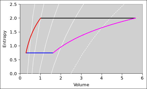
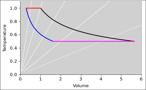
In this section, we do a preliminary analysis of the Carnot cycle. We carry out the analysis using two slightly different viewpoints, running both analyses in parallel. In figure 8.5 and figure 8.6 the physics is the same; only the presentation is different. The primary difference is the choice of axes: (V,T) versus (P,T). Every other difference can be seen as a consequence of this choice.
| In figure 8.5: | In figure 8.6: |
| When the engine is doing work we go clockwise around the cycle. | When the engine is doing work we go counterclockwise around the cycle. |
In other words, the sequence for positive work being done by the engine is this: red, black, magenta, blue.
|
| |
| Figure 8.5: Carnot Cycle : T versus V | Figure 8.6: Carnot Cycle : T versus P | |
In all of these figures, the contours of constant pressure are shown in white. The pressure values form a geometric sequence: {1/8, 1/4, 1/2, 1, 2}. In figure 8.6 this is obvious, but in the other figures you will just have to remember it. The P=1/8 contour is shown as a dotted line, to make it easy to recognize. The P=1 contour goes through the corner where red meets black.
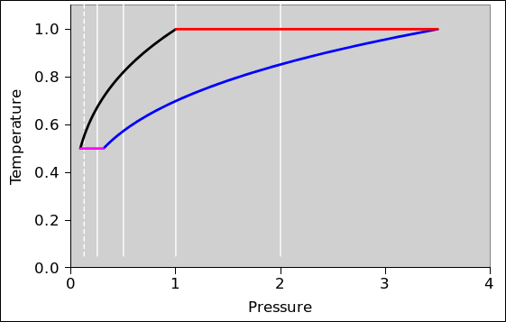
There are at least a dozen different ways of plotting this sort of data. Another version is shown in figure 8.7. It is somewhat remarkable that multiple figures portraying the same physics would look so different at first glance. I diagrammed the situation in multiple ways partly to show the difference, and partly to make – again – the point that any of the thermodynamic state-functions can be drawn as a function of any reasonable set of variables.
The spreadsheet used to compute these diagrams is cited in reference 24.
It’s interesting that we can replot the data in such a way as to change the apparent shape of the diagram ... without changing the meaning. This clarifies something that was mentioned in goal 5 in section 0.3: In thermodynamic state-space, there is a topology but not a geometry. We can measure the distance (in units of S) between contours of constant S, but we cannot compare that to any distance in any other direction.
In thermodynamics, there are often more variables than one can easily keep track of. Here we focus attention on T, V, P, and S. There are plenty of other variables (such as E) that we will barely even mention. Note that the number of variables far exceeds the number of dimensions. We say this is a two-dimensional situation, because it can be projected onto a two-dimensional diagram without losing any information.
It takes some practice to get the hang of interpreting these diagrams.
The Carnot cycle has four phases.
The amount of expansion is a design choice. In the example I arbitrarily chose a volume ratio of 3.5:1 for this phase of the expansion. (This is not the so-called “compression ratio” of the overall engine, since we have so far considered only one of the two compression phases.)
We continue the expansion until the temperature of the gas reaches the temperature of the low-temperature heat bath.
The amount of expansion required to achieve this depends on the gamma of the gas and (obviously) on the ratio of temperatures. For the example I assumed a 2:1 temperature ratio, which calls for a 5.7:1 expansion ratio during this phase. In general, for an adiabatic expansion, if you know the temperature ratio you can calculate the expansion ratio for this phase via
| (8.18) |
For the figures I used the gamma value appropriate for air and similar diatomic gases, namely γ = 7/5 = 1.4. A monatomic gas would need a significantly lower compression ratio for any given temperature ratio.
During the two expansion phases, the gas does work on the flywheel. During the two compression phases, the flywheel needs to do work on the gas. However, the compression-work is strictly less in magnitude than the expansion-work, so during the cycle net energy is deposited in the flywheel.
To understand this at the next level of detail, recall that mechanical work is −P dV. Now the integral of dV around the cycle is just ΔV which is zero. But what about the integral of P dV? Consider for example the step in V that goes from V=3 to V=4 along the black curve, and the corresponding step that goes from V=4 to V=3 along the magenta curve. The work done during the expansion phase (black) will be strictly greater than the work done during the recompression phase (magenta) because the pressure is higher. You can make the same argument for every piece of V in the whole V-space: For every ΔV in one of the expansion phases there will be a corresponding ΔV directly below it in one of the compression phases. For each of these pairs, expansion-work will be strictly greater than the compression-work because the pressure will be higher.
You can infer the higher pressure from the white contours of constant pressure, or you can just observe that the pressure must be higher because the temperature is higher.