25  Equipartition

25.1  Generalized Equipartition Theorem

In this chapter we temporarily lower our standards and derive some results that apply only in the classical limit, specifically in the “energy continuum” limit. That is, we assume that the temperature is high compared to the spacing between energy levels, so that when evaluating the partition function we can approximate the sum by an integral. We further assume that the system occupies a bounded region in phase space. That is, we assume there is zero probability that any of the position variables or momentum variables will ever take on super-large values.

Subject to these provisos, we¹ can write the partition function as:

Here we intend x and v to represent, somewhat abstractly, whatever variables contribute to the energy. (We imagine that x represents the variable or variables that contribute to the potential energy, while v represents the variable or variables that contribute to the kinetic energy, but this distinction is not important.)

Using 20/20 hindsight, we anticipate that it will be interesting to evaluate the expectation value of ∂E/∂ln(x) | v. We can evaluate this in the usual way, in terms of the partition function:

We now integrate by parts. The boundary terms vanish, because we have assumed the system occupies a bounded region in phase space.

We can of course write a corresponding result for the v-dependence at constant x:

and if there are multiple variables {x_i} and {v_i} we can write a corresponding result for each of them. This is called the generalized equipartition theorem.

25.2  Corollaries: Power-Law Equipartition

An interesting corollary is obtained in the case where the energy contains a power-law term of the form E_j = |x|^M:

In the very common case where M=2, this reduces to

and if the total energy consists of a sum of D such terms, the total energy is

This result is the quadratic corollary to the equipartition theorem. The symbol D_▯ (pronounced “D quad”) is the number of quadratic degrees of freedom of the system. Here we are assuming every degree of freedom appears in the Hamiltonian either quadratically or not at all.

All too often, equation 25.7 is called simply “the” equipartition theorem. However, we should beware that it it is only a pedestrian corollary. It only applies when every degree of freedom contributes to the energy either quadratically or not at all. This includes a remarkably large number of situations, including the harmonic oscillator, the particle in a box, and the rigid rotor ... but certainly not all situations, as discussed in section 25.3.

Also keep in mind that all the results in this chapter are based on the assumption that the system is classical, so that in the definition of the partition function we can approximate the sum by an integral.

25.3  Harmonic Oscillator, Particle in a Box, and Other Potentials

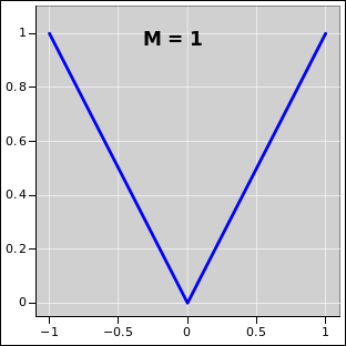
Let us consider a particle moving in one dimension in a power-law potential well. The energy is therefore

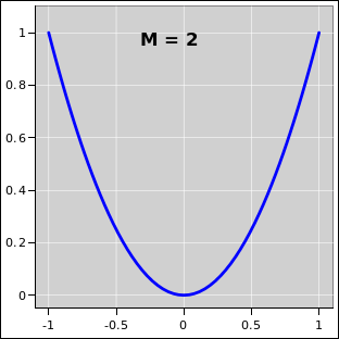
where the first term represents the usual kinetic energy (in some units) and the second term represents the potential energy. The case M=2 corresponds to a harmonic oscillator, as shown in figure 25.2.

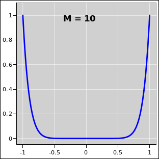
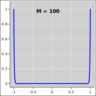
As M becomes larger and larger, the situation begins to more and more closely resemble a square-well potential, i.e. a particle in a box, as you can see in figure 25.3 and figure 25.4.

Figure 25.1: M = 1 i.e. Linear Power-Law Potential Well		Figure 25.2: M = 2 i.e. Quadratic Power-Law Potential Well

Figure 25.3: M = 10 Power-Law Potential Well		Figure 25.4: M = 100 Power-Law Potential Well

Let us apply the generalized equipartition theorem, namely equation 25.3 and equation 25.4, to each of these situations.

25.4  Remarks

It must be emphasized that every degree of freedom counts as a degree of freedom, whether or not it contributes to the heat capacity. For example, consider a free particle in three dimensions:

• For a one-dimensional harmonic oscillator, there are two quadratic degrees of freedom. Both contribute to the entropy, and both contribute to the energy.
• For the square well, there is only one quadratic degree of freedom, namely the one that gives rise to the kinetic energy. In contrast, the position is a non-quadratic degree of freedom, and contributes nothing to the average energy; there is no relevant potential energy.
• In the general case, you are not allowed to simply ignore non-quadratic degrees of freedom. In the example defined by equation 25.8, varying the exponent M from M=2 on up allows us to interpolate between the harmonic oscillator and the square well. At one extreme (M=2) the potential energy is quadratic, and at the other extreme (M=∞) the potential energy is irrelevant ... but in between, it is both relevant and non-quadratic.
• The M=1 case is easy to analyze, interesting, and reasonably common. For example, it applies to the m|g|h term in a tall column of gas in a gravitational field, as shown in figure 9.6.
• For any degree of freedom where the spacing between energy levels is large compared to kT, that degree of freedom contributes nothing very interesting to the average energy. (This is the polar opposite of the “energy continuum” limit.) We say that such a degree of freedom is “frozen out” by the laws of quantum mechanics.
• The idea of equipartion fails miserably for the spin system discussed in section 24.4, because the system does not have any quadratic degrees of freedom, and more importantly because the “energy continuum” approximation does not apply.
• Pedestrian ideas of equipartition can be applied to the ratio of specific heats of common gases, but only very imperfectly, as shown in table 26.1. This is because the “energy continuum” approximation applies to some of the degrees of freedom but not others. That is, some of the degrees of freedom have a moderately large spacing, so that they are quantum-mechanically “frozen out” at some temperatures but not others. For additional discussion of this point, see section 26.7.

1

This calculation in this section parallels Appendix G in M.D. Sturge, Statistical and Thermal Physics (2003)