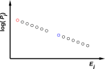
For reasons discussed in chapter 23, whenever a system is in thermal equilibrium, the energy is distributed among the microstates according to a very special probability distribution, namely the Boltzmann distribution. That is, the probability of finding the system in microstate i is given by:
| Pi = e−Êi / kT … for a thermal distribution (9.1) |
where Êi is the energy of the ith microstate, and kT is the temperature measured in energy units. That is, plain T is the temperature, and k is Boltzmann’s constant, which is just the conversion factor from temperature units to energy units.
Figure 9.1 shows this distribution graphically.
Evidence in favor of equation 9.1 is discussed in section 11.2.
When thinking about equation 9.1 and figure 9.1 it is important to realize that things don’t have to be that way. There are other possibilities. Indeed, a theory of thermodynamics that assumed that everything in sight was always in equilibrium at temperature T would be not worth the trouble. For starters, it is impossible to build a heat engine unless the hot reservoir is not in equilibrium with the cold reservoir.
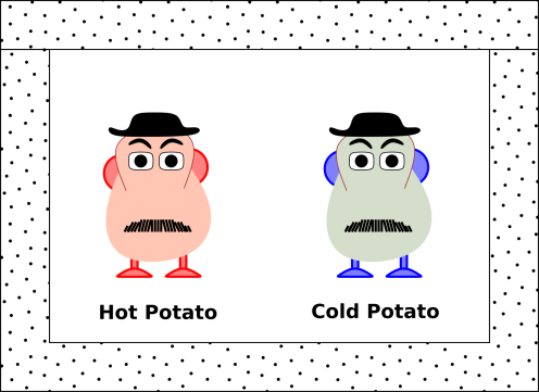
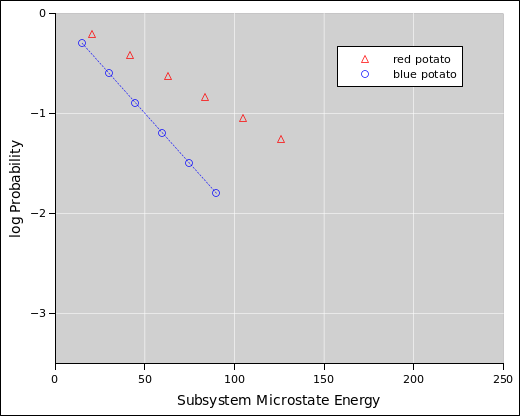
We start by considering the system shown in figure 9.2, namely a styrofoam box containing a hot potato and a cold potato. (This is a simplified version of figure 1.2.)
In situations like this, we can make good progress if we divide the system into subsystems. Here subsystem A is the red potato, and subsystem B is the blue potato. Each subsystem has a well defined temperature, but initially the system as a whole does not.
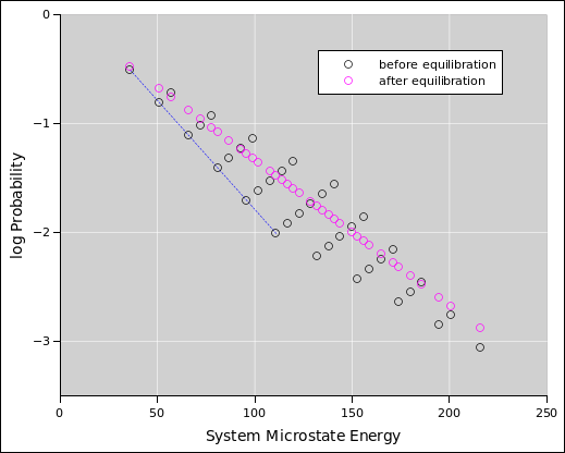
If we wait long enough, the two potatoes will come into equilibrium with each other, and at this point the system as a whole will have a well defined temperature. However, we are not required to wait for this to happen.
The difference between random energy and predictable energy has many consequences. The most important consequence is that the predictable energy can be freely converted to and from other forms, such as gravitational potential energy, chemical energy, electrical energy, et cetera. In many cases, these conversions can be carried out with very high efficiency. In some other cases, though, the laws of thermodynamics place severe restrictions on the efficiency with which conversions can be carried out, depending on to what extent the energy distribution deviates from the Boltzmann distribution.
Ironically, the first law of thermodynamics (equation 1.1) does not depend on temperature. Energy is well-defined and is conserved, no matter what. It doesn’t matter whether the system is hot or cold or whether it even has a temperature at all.
Even more ironically, the second law of thermodynamics (equation 2.1) doesn’t depend on temperature, either. Entropy is well-defined and is paraconserved no matter what. It doesn’t matter whether the system is hot or cold or whether it even has a temperature at all.
(This state of affairs is ironic because thermodynamics is commonly defined to be the science of heat and temperature, as you might have expected from the name: thermodynamics. Yet in our modernized and rationalized thermodynamics, the two most central, fundamental ideas – energy and entropy – are defined without reference to heat or temperature.)
Of course there are many important situations that do involve temperature. Most of the common, every-day applications of thermodynamics involve temperature – but you should not think of temperature as the essence of thermodynamics. Rather, it is a secondary concept which is defined (if and when it even exists) in terms of energy and entropy.
You may have heard the term “kinetic theory”. In particular, the thermodynamics of ideal gases is commonly called the kinetic theory of gases. However, you should be careful, because “kinetic theory” is restricted to ideal gases (indeed to a subset of ideal gases) ... while thermodynamics applies to innumerable other things. Don’t fall into the trap of thinking that there is such a thing as “thermal energy” and that this so-called “thermal energy” is necessarily kinetic energy. In almost all systems, including solids, liquids, non-ideal gases, and even some ideal gases, the energy is a mixture of kinetic and potential energy. (Furthermore, in any non-cramped situation, i.e. in any situation where it is possible to build a heat engine, it is impossible in principle to define any such thing as “thermal energy”.) In any case, it is safer and in all ways better to say thermodynamics or statistical mechanics instead of “kinetic theory”.
In typical systems, potential energy and kinetic energy play parallel roles:
In fact, for an ordinary crystal such as quartz or sodium chloride, almost exactly half of the heat capacity is due to potential energy, and half to kinetic energy. It’s easy to see why that must be: The heat capacity is well described in terms of thermal phonons in the crystal. Each phonon mode is a harmonic1 oscillator. In each cycle of any harmonic oscillator, the energy changes from kinetic to potential and back again. The kinetic energy goes like sin2(phase) and the potential energy goes like cos2(phase), so on average each of those is half of the total energy.
| |
A table-top sample of ideal gas is a special case, where all the energy is kinetic energy. This is very atypical of thermodynamics in general. Table-top ideal gases are very commonly used as an illustration of thermodynamic ideas, which becomes a problem when the example is overused so heavily as to create the misimpression that thermodynamics deals only with kinetic energy.
You could argue that in many familiar systems, the temperature is closely related to random kinetic energy ... but temperature is not the same thing as so-called “heat’ or “thermal energy”. Furthermore, there are other systems, such as spin systems, where the temperature is not related to the random kinetic energy.
All in all, it seems quite unwise to define heat or even temperature in terms of kinetic energy.
This discussion continues in section 9.3.4.
We have seen that for an ideal gas, there is a one-to-one correspondence between the temperature and the kinetic energy of the gas particles. However, that does not mean that there is a one-to-one correspondence between kinetic energy and heat energy. (In this context, heat energy refers to whatever is measured by a heat capacity experiment.)
To illustrate this point, let’s consider a sample of pure monatomic nonrelativistic nondegenerate ideal gas in a tall cylinder of horizontal radius r and vertical height h at temperature T. The pressure measured at the bottom of the cylinder is P. Each particle in the gas has mass m. We wish to know the heat capacity per particle at constant volume, i.e. CV/N.
At this point you may already have in mind an answer, a simple answer, a well-known answer, independent of r, h, m, P, T, and N. But wait, there’s more to the story: The point of this exercise is that h is not small. In particular, m|g|h is not small compared to kT, where g is the acceleration of gravity. For simplicity, you are encouraged to start by considering the limit where h goes to infinity, in which case the exact value of h no longer matters. Gravity holds virtually all the gas near the bottom of the cylinder, whenever h ≫ kT/m|g|.
You will discover that a distinctly nontrivial contribution to the heat capacity comes from the potential energy of the ideal gas. When you heat it up, the gas column expands, lifting its center of mass, doing work against gravity. (Of course, as always, there will be a contribution from the kinetic energy.)
For particles the size of atoms, the length-scale kT/m|g| is on the order of several kilometers, so the cylinder we are considering is much too big to fit on a table top. I often use the restrictive term “table-top” as a shorthand way of asserting that m|g|h is small compared to kT.
So, this reinforces the points made in section 9.3.3. We conclude that in general, heat energy is not just kinetic energy.
Beware that this tall cylinder is not a good model for the earth’s atmosphere. For one thing, the atmosphere is not isothermal. For another thing, if you are going to take the limit as h goes to infinity, you can’t use a cylinder; you need something more like a cone, spreading out as it goes up, to account for the spherical geometry.
Over the years, lots of people have noticed that you can always split the kinetic energy of a complex object into the KE of the center-of-mass motion plus the KE of the relative motion (i.e. the motion of the components relative to the center of mass).
Also a lot of people have tried (with mixed success) to split the energy of an object into a “thermal” piece and a “non-thermal” piece.
It is an all-too-common mistake to think that the overall/relative split is the same as the nonthermal/thermal split. Beware: they’re not the same. Definitely not. See section 7.7 for more on this.
First of all, the microscopic energy is not restricted to being kinetic energy, as discussed in section 9.3.3. So trying to understand the thermal/non-thermal split in terms of kinetic energy is guaranteed to fail. Using the work/KE theorem (reference 18) to connect work (via KE) to the thermal/nonthermal split is guaranteed to fail for the same reason.
Secondly, a standard counterexample uses flywheels, as discussed in section 18.4. You can impart macroscopic, non-Locrian KE to the flywheels without imparting center-of-mass KE or any kind of potential energy … and without imparting any kind of Locrian energy (either kinetic or potential).
The whole idea of “thermal energy” is problematic, and in many cases impossible to define, as discussed in chapter 19. If you find yourself worrying about the exact definition of “thermal energy”, it means you’re trying to solve the wrong problem. Find a way to reformulate the problem in terms of energy and entropy.
Center-of-mass motion is an example but not the only example of low-entropy energy. The motion of the flywheels is one perfectly good example of low-entropy energy. Several other examples are listed in section 11.3.
A macroscopic object has something like 1023 modes. The center-of-mass motion is just one of these modes. The motion of counter-rotating flywheels is another mode. These are slightly special, but not very special. A mode to which we can apply a conservation law, such as conservation of momentum, or conservation of angular momentum, might require a little bit of special treatment, but usually not much … and there aren’t very many such modes.
Sometimes on account of conservation laws, and sometimes for other reasons as discussed in section 11.11 it may be possible for a few modes of the system to be strongly coupled to the outside (and weakly coupled to the rest of the system), while the remaining 1023 modes are more strongly coupled to each other than they are to the outside. It is these issues of coupling-strength that determine which modes are in equilibrium and which (if any) are far from equilibrium. This is consistent with our definition of equilibrium (section 10.1).
Thermodynamics treats all the equilibrated modes on an equal footing. One manifestation of this can be seen in equation 9.1, where each state contributes one term to the sum … and addition is commutative.
There will never be an axiom that says such-and-such mode is always in equilibrium or always not; the answer is sensitive to how you engineer the couplings.
It is a common mistake to visualize entropy as a highly dynamic process, whereby the system is constantly flipping from one microstate to another. This may be a consequence of the fallacy discussed in section 9.3.5 (mistaking the thermal/nonthermal distinction for the kinetic/potential distinction) … or it may have other roots; I’m not sure.
In any case, the fact is that re-shuffling is not an essential part of the entropy picture.
An understanding of this point proceeds directly from fundamental notions of probability and statistics.
By way of illustration, consider one hand in a game of draw poker.
Let’s more closely examine step (B). At this point you have to make a decision based on probability. The deck, as it sits there, is not constantly re-arranging itself, yet you are somehow able to think about the probability that the card you draw will complete your inside straight.
The deck, as it sits there during step (B), is not flipping from one microstate to another. It is in some microstate, and staying in that microstate. At this stage you don’t know what microstate that happens to be. Later, at step (C), long after the hand is over, you might get a chance to find out the exact microstate, but right now at step (B) you are forced to make a decision based only on the probability.
The same ideas apply to the entropy of a roomful of air, or any other thermodynamic system. At any given instant, the air is in some microstate with 100% probability; you just don’t know what microstate that happens to be. If you did know, the entropy would be zero … but you don’t know. You don’t need to take any sort of time-average to realize that you don’t know the microstate.
The bottom line is that the essence of entropy is the same as the essence of probability in general: The essential idea is that you don’t know the microstate. Constant re-arrangement is not essential.
This leaves us with the question of whether re-arrangement is ever important. Of course the deck needs to be shuffled at step (A). Not constantly re-shuffled, just shuffled the once.
Again, the same ideas apply to the entropy of a roomful of air. If you did somehow obtain knowledge of the microstate, you might be interested in the timescale over which the system re-arranges itself, making your erstwhile knowledge obsolete and thereby returning the system to a high-entropy condition.
The crucial point remains: the process whereby knowledge is lost and entropy is created is not part of the definition of entropy, and need not be considered when you evaluate the entropy. If you walk into a room for the first time, the re-arrangement rate is not your concern. You don’t know the microstate of this room, and that’s all there is to the story. You don’t care how quickly (if at all) one unknown microstate turns into another.
If you don’t like the poker analogy, we can use a cryptology analogy instead. Yes, physics, poker, and cryptology are all the same when it comes to this. Statistics is statistics.
If I’ve intercepted just one cryptotext from the opposition and I’m trying to crack it, on some level what matters is whether or not I know their session key. It doesn’t matter whether that session key is 10 microseconds old, or 10 minutes old, or 10 days old. If I don’t have any information about it, I don’t have any information about it, and that’s all that need be said.
On the other hand, if I’ve intercepted a stream of messages and extracted partial information from them (via a partial break of the cryptosystem), the opposition would be well advised to “re-shuffle the deck” i.e. choose new session keys on a timescale fast compared to my ability to extract information about them.
Applying these ideas to a roomful of air: Typical sorts of measurements give us only a pathetically small amount of partial information about the microstate. So it really doesn’t matter whether the air re-arranges itself super-frequently or super-infrequently. We don’t have any significant amount of information about the microstate, and that’s all there is to the story.
Reference 25 presents a simulation that demonstrates the points discussed in this subsection.
Before we go any farther, convince yourself that
| (9.2) |
and in general, multiplying a logarithm by some positive number corresponds to changing the base of the logarithm.
In the formula for entropy, equation 2.2, the base of the logarithm has intentionally been left unspecified. You get to choose a convenient base. This is the same thing as choosing what units will be used for measuring the entropy.
Some people prefer to express the units by choosing the base of the logarithm, while others prefer to stick with natural logarithms and express the units more directly, using an expression of the form:
| S[P] := k |
| Pi ln(1/Pi) (9.3) |
In this expression we stipulated e as the base of the logarithm. Whereas equation 2.2 we could choose the base of the logarithm, in equation 9.3 we get to choose the numerical value and units for k. This is a superficially different solution to the same problem. Reasonable choices include:
| (9.4) |
It must be emphasized that all these expressions are mathematically equivalent. In each case, the numerical part of k balances the units of k, so that the meaning remains unchanged. In some cases it is convenient to absorb the numerical part of k into the base of the logarithm:
| (9.5) |
where the third line uses the remarkably huge base Ω = exp(1.24×10²²). When dealing with smallish amounts of entropy, units of bits are conventional and often convenient. When dealing with large amounts of entropy, units of J/K are conventional and often convenient. These are related as follows:
| (9.6) |
A convenient unit for molar entropy is Joules per Kelvin per mole:
| (9.7) |
Values in this range (on the order of one bit per particle) are very commonly encountered.
If you are wondering whether equation 9.7 is OK from a dimensional-analysis point of view, fear not. Temperature units are closely related to energy units. Specifically, energy is extensive and can be measured in joules, while temperature is intensive and can be measured in kelvins. Therefore combinations such as (J/K/mol) are dimensionless units. A glance at the dimensions of the ideal gas law should suffice to remind you of this if you ever forget.See reference 26 for more about dimensionless units.
Let us spend a few paragraphs discussing a strict notion of multiplicity, and then move on to a more nuanced notion. (We also discuss the relationship between an equiprobable distribution and a microcanonical ensemble.)
Suppose we have a system where a certain set of states2 (called the “accessible” states) are equiprobable, i.e. Pi = 1/W for some constant W. Furthermore, all remaining states are “inaccessible” which means they all have Pi = 0. The constant W is called the multiplicity.
Note: Terminology: The W denoting multiplicity in this section is unrelated to the W denoting work elsewhere in this document. Both usages of W are common in the literature. It is almost always obvious from context which meaning is intended, so there isn’t a serious problem. Some of the literature uses Ω to denote multiplicity.
The probability per state is necessarily the reciprocal of the number of accessible states, since (in accordance with the usual definition of “probability”) we want our probabilities to be normalized: ∑ Pi = 1.
In this less-than-general case, the entropy (as given by equation 2.2) reduces to
| S = logW (provided the microstates are equiprobable) (9.8) |
As usual, you can choose the base of the logarithm according to what units you prefer for measuring entropy: bits, nats, trits, J/K, or whatever. Equivalently, you can fix the base of the logarithm and express the units by means of a factor of k out front, as discussed in section 9.5:
| S = k lnW (provided the microstates are equiprobable) (9.9) |
This equation is prominently featured on Boltzmann’s tombstone. However, I’m pretty sure (a) he didn’t put it there, (b) Boltzmann was not the one who originated or emphasized this formula (Planck was), and (c) Boltzmann was well aware that this is not the most general expression for the entropy. I mention this because a lot of people who ought to know better take equation 9.9 as the unassailable definition of entropy, and sometimes they cite Boltzmann’s tombstone as if it were the ultimate authority on the subject.In any case, (d) even if Boltzmann had endorsed equation 9.9, appeal to authority is not an acceptable substitute for scientific evidence and logical reasoning. We know more now than we knew in 1898, and we are allowed to change our minds about things ... although in this case it is not necessary. Equation 2.2 has been the faithful workhorse formula for a very long time.
There are various ways a system could wind up with equiprobable states:
Consider two blocks of copper that are identical except that one of them has more energy than the other. They are thermally isolated from each other and from everything else. The higher-energy block will have a greater number of accessible states, i.e. a higher multiplicity. In this way you can, if you wish, define a notion of multiplicity as a function of energy level.
On the other hand, you must not get the idea that multiplicity is a monotone function of energy or vice versa. Such an idea would be quite incorrect when applied to a spin system.
Terminology: By definition, a level is a group of microstates. An energy level is a group of microstates all with the same energy (or nearly the same energy, relative to other energy-scales in the problem). By connotation, usually when people speak of a level they mean energy level.
We now introduce a notion of “approximate” equiprobability and “approximate” multiplicity by reference to the example in the following table:
| Level | | # microstates | Probability | Probability | Entropy |
| | in level | of microstate | of level | (in bits) | |
| 1 | | 2 | 0.01 | 0.020 | 0.133 |
| 2 | | 979 | 0.001 | 0.989 | 9.757 |
| 3 | | 1,000,000 | 1E-09 | 0.001 | 0.030 |
| Total: | | 1,000,981 | 1.000 | 9.919 | |
The system in this example 1,000,981 microstates, which we have grouped into three levels. There are a million states in level 3, each of which occurs with probability one in a billion, so the probability of observing some state from this level is one in a thousand. There are only two microstates in level 1, each of which is observed with a vastly larger probability, namely one in a hundred. Level 2 is baby-bear just right. It has a moderate number of states, each with a moderate probability ... with the remarkable property that on a level-by-level basis, this level dominates the probability distribution. The probability of observing some microstate from level 2 is nearly 100%.
The bottom line is that the entropy of this distribution is 9.919 bits, which is 99.53% of the entropy you would have if all the probability were tied up in 1000 microstates with probability 0.001 each.
Beware of some overloaded terminology:
| In the table, the column we have labeled “# microstates in level” is conventionally called the multiplicity of the level. | If we apply the S = log(W) formula in reverse, we find that our example distribution has a multiplicity of W = 2S = 29.919 = 968; this is the effective multiplicity of the distribution as a whole. |
So we see that the effective multiplicity of the distribution is dominated by the multiplicity of level 2. The other levels contribute very little to the entropy.
You have to be careful how you describe the microstates in level 2. Level 2 is the most probable level (on a level-by-level basis), but its microstates are not the most probable microstates (on a microstate-by-microstate basis).
In the strict notion of multiplicity, all the states that were not part of the dominant level were declared “inaccessible”, but alas this terminology becomes hopelessly tangled when we progress to the nuanced notion of multiplicity. In the table, the states in level 3 are high-energy states, and it might be OK to say that they are energetically inaccessible, or “almost” inaccessible. It might be superficially tempting to label level 1 as also inaccessible, but that would not be correct. The states in level 1 are perfectly accessible; their only problem is that they are few in number.
I don’t know how to handle “accessibility” except to avoid the term, and to speak instead of “dominant” levels and “negligible” levels.
| A system that is thermally isolated so that all microstates have the same energy is called microcanonical. | In contrast, an object in contact with a constant-temperature heat bath is called canonical (not microcanonical). Furthermore, a system that can exchange particles with a reservoir, as described by a chemical potential, is called grand canonical (not microcanonical or canonical). |
| The strict definition of multiplicity applies directly to microcanonical ensembles and other strictly equiprobable distributions. Equation 9.8 applies exactly to such systems. | Equation 9.8 does not apply exactly to canonical or grand-canonical systems, and may not apply even approximately. The correct thermal probability distribution is shown in figure 9.1. |
| There exist intermediate cases, which are common and often important. In a canonical or grand-canonical thermal system, we can get into a situation where the notion of multiplicity is a good approximation – not exact, but good enough. This can happen if the energy distribution is so strongly peaked near the most-probable energy that the entropy is very nearly what you would get in the strictly-equiprobable case. This can be roughly understood in terms of the behavior of Gaussians. If we combine N small Gaussians to make one big Gaussian, the absolute width scales like √N and the relative width scales like √N/N. The latter is small when N is large. |
One should not attach too much importance to the tradeoff in the table above, namely the tradeoff between multiplicity (increasing as we move down the table) and per-microstate probability (decreasing as we move down the table). It is tempting to assume all thermal systems must involve a similar tradeoff, but they do not. In particular, at negative temperatures (as discussed in reference 27), it is quite possible for the lower-energy microstates to outnumber the higher-energy microstates, so that both multiplicity and per-microstate probability are decreasing as we move down the table toward higher energy.
You may reasonably ask whether such a system might be unstable, i.e. whether the entire system might spontaneously move toward the high-energy high-probability high-multiplicity state. The answer is that such a move cannot happen because it would not conserve energy. In a thermally-isolated system, if half of the system moved to higher energy, you would have to “borrow” that energy from the other half, which would then move to lower energy, lower multiplicity, and lower probability per microstate. The overall probability of the system depends on the probability of the two halves taken jointly, and this joint probability would be unfavorable. If you want to get technical about it, stability does not depend on the increase or decrease of multiplicity as a function of energy, but rather on the convexity which measures what happens if you borrow energy from one subsystem and lend it to another.
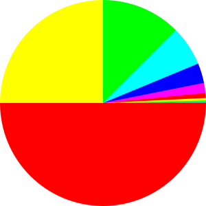
Consider the probability distribution shown in figure 9.5. There is one microstate with probability 1/2, another with probability 1/4, another with probability 1/8, et cetera. Each microstate is represented by a sector in the diagram, and the area of the sector is proportional to the microstate’s probability.
Some information about these microstates can be found in the following table.
| State# | Probability | Suprise Value |
| / bits | ||
| 1 | 0.5 | 1 |
| 2 | 0.25 | 2 |
| 3 | 0.125 | 3 |
| 4 | 0.0625 | 4 |
| 5 | 0.03125 | 5 |
| 6 | 0.015625 | 6 |
| 7 | 0.0078125 | 7 |
| 8 | 0.00390625 | 8 |
| 9 | 0.001953125 | 9 |
| 10 | 0.0009765625 | 10 |
| ... | et cetera | ... |
The total probability adds up to 1, as you can verify by summing the numbers in the middle column. The total entropy is 2, as you can verify by summing the surprisals weighted by the corresponding probabilities. The total number of states is infinite, and the multiplicity W is infinite. Note that
| (9.10) |
which means that equation 9.9 definitely fails to work for this distribution. It fails by quite a large margin.
Some people are inordinately fond of equation 9.8 or equivalently equation 9.9. They are tempted to take it as the definition of entropy, and sometimes offer outrageously unscientific arguments in its support. But the fact remains that Equation 2.2 is an incomparably more general, more reliable expression, while equation 9.9 is a special case, a less-than-general corollary, a sometimes-acceptable approximation.
Specific reasons why you should not consider equation 9.8 to be axiomatic include:
For a thermal distribution, the probability of a microstate is given by equation 9.1. So, even within the restricted realm of thermal distributions, equation 9.9 does not cover all the bases; it applies if and only if all the accessible microstates have the same energy. It is possible to arrange for this to be true, by constraining all accessible microstates to have the same energy. That is, it is possible to create a microcanonical system by isolating or insulating and sealing the system so that no energy can enter or leave. This can be done, but it places drastic restrictions on the sort of systems we can analyze.
This section exists mainly to dispel a misconception. If you do not suffer from this particular misconception, you should probably skip this section, especially on first reading.
Non-experts sometimes get the idea that whenever something is more dispersed – more spread out in position – its entropy must be higher. This is a mistake.
There is a fundamental conceptual problem, which should be obvious from the fact that the degree of dispersal, insofar as it can be defined at all, is a property of the microstate – whereas entropy is a property of the macrostate as a whole, i.e. a property of the ensemble, i.e. a property of the probability distribution as a whole, as discussed in section 2.4 and especially section 2.7.1. A similar microstate versus macrostate argument applies to the “disorder” model of entropy, as discussed in section 2.5.5. In any case, whatever “dispersal” is measuring, it’s not entropy.
Yes, you can find selected scenarios where a gas expands and the system does gain entropy (such as isothermal expansion, or diffusive mixing as discussed in section 11.6) … but there are also scenarios where a gas expands but the system does not gain entropy (reversible thermally-isolated expansion). Indeed there are scenarios where a system gains entropy when the gas becomes less spread out, as we now discuss:
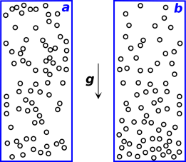
Consider a closed system consisting of a tall column of gas in a gravitational field, at a uniform not-too-high temperature such that kT < m|g|H. Start from a situation where the density3 is uniform, independent of height, as in figure 9.6a. This is not the equilibrium distribution.
As the system evolves toward equilibrium, irreversibly, its entropy will increase. At equilibrium, the density will be greater toward the bottom and lesser toward the top, as shown in figure 9.6b. Furthermore, the equilibrium situation does not exhibit even dispersal of energy. The kinetic energy per particle is evenly dispersed, but the potential energy per particle and the total energy per particle are markedly dependent on height.
There are theorems about what does get uniformly distributed, as discussed in chapter 25. Neither density nor energy is the right answer.
As another example, consider two counter-rotating flywheels. In particular, imagine that these flywheels are annular in shape, i.e. hoops, as shown in figure 9.7, so that to a good approximation, all the mass is at the rim, and every bit of mass is moving at the same speed. Also imagine that they are stacked on the same axis. Now let the two wheels rub together, so that friction causes them to slow down and heat up. Entropy has been produced, but the energy has not become more spread-out in space. To a first approximation, the energy was everywhere to begin with and everywhere afterward, so there is no change.
If we look more closely, we find that as the entropy increased, the energy dispersal actually decreased slightly. That is, the energy became slightly less evenly distributed in space. Under the initial conditions, the macroscopic rotational mechanical energy was evenly distributed, and the microscopic forms of energy were evenly distributed on a macroscopic scale, plus or minus small local thermal fluctuations. Afterward, the all the energy is in the microscopic forms. It is still evenly distributed on a macroscopic scale, plus or minus thermal fluctuations, but the thermal fluctuations are now larger because the temperature is higher. Let’s be clear: If we ignore thermal fluctuations, the increase in entropy was accompanied by no change in the spatial distribution of energy, while if we include the fluctuations, the increase in entropy was accompanied by less even dispersal of the energy.
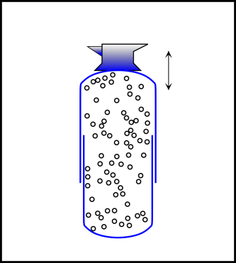
Here’s yet another nail in the coffin of the «dispersal» model of entropy. Consider a thermally isolated system consisting of gas in a piston pushing up on a mass, subject to gravity, as shown in figure 9.8. Engineer it to make dissipation negligible. Let the mass oscillate up and down, reversibly. The matter and energy become repeatedly more and less «disperse», with no change in entropy.
Here’s another reason why any attempt to define entropy in terms of “energy dispersal” or the like is Dead on Arrival: Entropy is defined in terms of probability, and applies to systems where the energy is zero, irrelevant, and/or undefinable.
As previously observed, states are states; they are not necessarily energy states.
You can salvage the idea of spreading if you apply it to the spreading of probability in an abstract probability-space (not the spreading of energy of any kind, and not spreading in ordinary position-space).
This is not the recommended way to introduce the idea of entropy, or to define entropy. It is better to introduce entropy by means of guessing games, counting the number of questions, estimating the missing information, as discussed in chapter 2. At the next level of detail, the workhorse formula for quantifying the entropy is equation 2.2This section exists mainly to dispel some spreading-related misconceptions. If you do not suffer from these particular misconceptions, you should probably skip this section, especially on first reading.
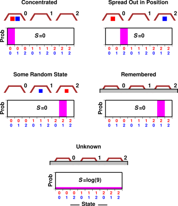
If you insist on using the idea of spreading, here’s an example that illustrates the idea and can be analyzed in detail. Figure 9.9 shows two blocks under three transparent cups. In the first scenario, the blocks are “concentrated” in the 00 state. In the probability histogram below the cups, there is unit probability (shown in magenta) in the 00 slot, and zero probability in the other slots, so p log(1/p) is zero everywhere. That means the entropy is zero.
In the next scenario, the blocks are spread out in position, but since we know exactly what state they are in, all the probability is in the 02 slot. That means p log(1/p) is zero everywhere, and the entropy is still zero.
In the third scenario, the system is in some randomly chosen state, namely the 21 state, which is as disordered and as random as any state can be, yet since we know what state it is, p log(1/p) is zero everywhere, and the entropy is zero.
The fourth scenario is derived from the third scenario, except that the cups are behind a screen. We can’t see the blocks right now, but we remember where they are. The entropy remains zero.
Finally, in the fifth scenario, we simply don’t know what state the blocks are in. The blocks are behind a screen, and have been shuffled since the last time we looked. We have some vague notion that on average, there is 2/3rds of a block under each cup, but that is only an average over many states. The probability histogram shows there is a 1-out-of-9 chance for the system to be in any of the 9 possible states, so ∑ p log(1/p) = log(9) .
One point to be made here is that entropy is not defined in terms of particles that are spread out (“dispersed”) in position-space, but rather in terms of probability that is spread out in state-space. This is quite an important distinction. For more details on this, including an interactive simulation, see reference 25.
| |
To use NMR language, entropy is produced on a timescale τ2, while energy-changes take place on a timescale τ1. There are systems where τ1 is huuugely longer than τ2. See also section 11.5.5 and figure 1.3. (If this paragraph doesn’t mean anything to you, don’t worry about it.)
As a way of reinforcing this point, consider a system of spins such as discussed in section 11.10. The spins change orientation, but they don’t change position at all. Their positions are locked to the crystal lattice. The notion of entropy doesn’t require any notion of position; as long as we have states, and a probability of occupying each state, then we have a well-defined notion of entropy. High entropy means the probability is spread out over many states in state-space.
State-space can sometimes be rather hard to visualize. As mentioned in section 2.3, a well-shuffled card deck has nearly 2226 bits of entropy … which is a stupendous number. If you consider the states of gas molecules in a liter of air, the number of states is even larger – far, far beyond what most people can visualize. If you try to histogram these states, you have an unmanageable number of slots (in contrast to the 9 slots in figure 9.9) with usually a very small probability in each slot.
Another point to be made in connection with figure 9.9 concerns the relationship between observing and stirring (aka mixing, aka shuffling). Here’s the rule:
| not looking | looking | |
| not stirring | entropy constant | entropy decreasing (aa) |
| stirring | entropy increasing (aa) | indeterminate change in entropy |
where (aa) means almost always; we have to say (aa) because entropy can’t be increased by stirring if it is already at its maximum possible value, and it can’t be decreased by looking if it is already zero. Note that if you’re not looking, lack of stirring does not cause an increase in entropy. By the same token, if you’re not stirring, lack of looking does not cause a decrease in entropy. If you are stirring and looking simultaneously, there is a contest between the two processes; the entropy might decrease or might increase, depending on which process is more effective.
The simulation in reference 25 serves to underline these points.
Last but not least, it must be emphasized that spreading of probability in probability-space is dramatically different from spreading energy (or anything else) in ordinary position-space. For one thing, these two spaces don’t even have the same size. Suppose you have a crystal with a million evenly-spaced copper atoms. We consider the magnetic energy of the nuclear spins. Each nucleus can have anywhere from zero to four units of energy. Suppose the total energy is two million units, which is what we would expect for such a system at high temperature.
Let’s be clear: a number with 600,000 digits is very much larger than a number with six or seven digits. If you imagine spreading the energy in position-space, it gives entirely the wrong picture. The physics cares about spreading the probability in a completely different space, a very much larger space. The probability is spread very much more thinly.