In this chapter, we consider the partition function for various interesting systems. We start with a single particle in a box (section 26.1. We then consider an ideal gas of N particles in a box (section 26.2), including a pure monatomic gas and mixtures of monatomic gases. We then consider the rigid rotor, as a model of a lightweight diatomic model (section 26.3). We use the partition function to derive some classic macroscopic thermodynamic formulas.
As discussed in section 26.9, the canonical partition function for a single high-temperature nonrelativistic pointlike particle in a box is:
| (26.1) |
where V is the volume of the container. The subscript “ppb” stands for “point particle in a box”. The RHS is temperature-dependent because Λ scales like √β. Here Λ is the thermal de Broglie length
| Λ := √( |
| ) (26.2) |
which is the same as equation 12.2.
In general, the partition function is defined in terms of an infinite series, but in many cases it is possible to sum the series. In this case the result is a compact, closed-form expression, namely equation 26.1.
Using partition functions is more fun than deriving them, so let’s start by doing some examples using equation 26.1, and postpone the derivation to section 26.9.
There’s a lot more we could say about this, but it’s easier to do the more-general case of the ideal gas (section 26.2) and treat the single particle in a box as a special case thereof, i.e. the N=1 case.
In this section, we generalize the single-particle partition function to a gas of multiple particles. We continue to assume all the particles are pointlike. At not-to-high temperatures, this is a good model for a monatomic gas.
We start by considering a single gas particle, and model it as a six-sided die. Since there are six possible states, the single-particle partition function has six terms:
| (26.3) |
We do not assume the die is fair, so the terms are not necessarily equal.
We now proceed to the case of N=2 dice. The partition function will have 62=36 terms. We can calculate the probability of each two-particle state in terms of the corresponding one-particle states. In fact, since the gas is ideal, each particle is independent of the other, so the single-particle probabilities are statistically independent, so each two-particle probability is just a simple product, as shown in the following equation:
| (26.4) |
where Q is the partition function for the first die, R is the partition function for the second die, and subscripts on Q and R identify terms within each single-particle partition function.
Using the distributive rule, we can simplify equation 26.4 quite a bit: we find simply Z=QR. If we now assume that the two dice are statistically the same (to a good approximation), then we can further simplify this to Z=Q2 (to the same good approximation). In the case of N dice, the general result is:
| Zdice|D = ( |
| ) | N (26.5) |
This is the correct result for the case where each particle has (almost) the same single-particle partition function, provided the particles remain enough different to be distinguishable in the quantum-mechanical sense ... and provided we know in advance which particles are going to appear in the mixture, so that there is no entropy of the deal (as defined in section 12.10).
We now consider a situation that is the same as above, except that the particles are all identical in the quantum-mechanical sense. (We will consider mixtures in section 26.2.3.) If we apply equation 26.4 to this situation, every term below the diagonal has a mirror-image term above the diagonal the describes exactly the same state. For example, Q2 R6 is the exact same state as Q6 R2. Therefore if we include all the terms in equation 26.4 in our sum over states, we have overcounted these off-diagonal states by a factor of two. So to a first approximation, neglecting the diagonal terms, we can correct for this by writing Z = QR/2. Generalizing from N=2 to general N, we have:
| (26.6) |
At the next level of detail, we should think a little more carefully about the diagonal terms in equation 26.4. There are two possibilities:
On the other hand, by hypothesis we are restricting attention to nondegenerate gases; therefore the chance of any particular slot being occupied is small, and the chance of any particular slot being occupied more than once is small squared, or smaller. That means there must be many, many terms in the sum over states, and the diagonal terms must be a small fraction of the total. Therefore we don’t much care what we do with the diagonal terms. We could keep them all, discard them all, or whatever; it doesn’t much matter. As N becomes larger, the diagonal terms become even less of a problem. The simplest thing is to arbitrarily use equation 26.6, which will be slightly too high for fermions and slightly too low for bosons, but close enough for most applications, provided the system really is nondegenerate.
Things get even more interesting when we consider mixtures.
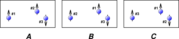
Figure 26.1 shows three particles that are very very nearly identical. In particular, this could represent three atoms of 3He, where arrows in the diagram represent the nuclear spins. There are six ways of labeling these three particles, of which three ways are shown in the figure.
In fact diagram A and diagram B depict exactly the same state. Particle #1 and particle #2 are quantum-mechanically identical, so the physics doesn’t care which is which. That is, these two labels are different only in our imagination.
Tangential technical remark: In a snapshot such as we see in figure 26.1, it could be argued that particle #1 and particle #2 are distinguishable by their positions, even though they are “identical” particles. Note that we are using some subtle terminology: identical is not the same as indistinguishable. The idea of “distinguishable by position" is valid at not-too-low temperatures, where the thermal de Broglie length is small compared to the spacing between particles. However, even in the best case it is only valid temporarily, because of the uncertainty principle: The more precisely we know the position at the present time, the less precisely we will know it at future times. For a minimum-uncertainty wave packet, the formula is
Δt =
2 m Δx2 ℏ (26.7)
which for atoms at ordinary atmospheric density is on the order of a nanosecond. This is much shorter than the timescale for carrying out a typical Gibbs-type mixing experiment, so under these conditions we should not think of the atoms as being distinguishable by position. (For a very dilute gas of massive particles on very fast timescales, the story might be different.)
The notion of “distinguishable by position” is sometimes important. Without it, classical physics would not exist. In particular, we would never be able to talk about an individual electron; we would be required to antisymmetrize the wavefunction with respect to every electron in the universe.
When we evaluate the partition function, each state needs to appear once and only once in the sum over states. In figure 26.1, we need to include A or B but not both, since they are two ways of describing the exact same state.
As is so often the case, we may find it convenient to count the states as if the particles were labeled, and then apply the appropriate delabeling factors.
For the gas shown in figure 26.1, we have N=3. The delabeling factor will be 2! for the spin-up component of the mixture, because there are 2 particles in this component. The delabeling factor will be 1! for the spin-down component, because there is only one particle in this component. For general N, if we assume that all the particles have the same single-particle partition function – which is what happens when the Hamiltonian is spin-independent – then the partition function for the gas as a whole is
| (26.8) |
where the index j runs over all components in the mixture. To derive the second line we have used the obvious sum rule for the total number of particles:
| Nj = N (26.9) |
The last line of equation 26.8 is very similar to equation 26.6, in the sense that both contain a factor of (V/Λ3) to the Nth power. Only the delabeling factors are different.
We can use equation 26.6 to find the energy for the pure gas, with the help of equation 24.9. Plugging in, we find
| (26.10) |
as expected for the ideal monatomic nondegenerate nonrelativistic pure gas in three dimensions. (See equation 26.42 for a more general expression, applicable to a polytropic gas. See section 26.2.3 for a discussion of mixtures, including mixtures of isotopes, mixtures of spin-states, et cetera.)
If you’re clever, you can do this calculation in your head, because the RHS of equation 26.6 depends on β to the −3N/2 power, and all the other factors drop out when you take the logarithmic derivative.
Note that equation 26.10 naturally expresses the energy as a function of temperature, in contrast to (say) equation 7.8 which treats the energy as a function of entropy. There is nothing wrong with either way of doing it. Indeed, it is best to think in topological terms, i.e. to think of energy at each point in thermodynamic state-space. We can describe this point in terms of its temperature, or in terms of its entropy, or in innumerable other ways.
This expression for the energy is independent of V. On the other hand, we are free to treat it a function of V (as well as T). We could multiply the RHS by V0, which is, formally speaking, a function of V, even though it isn’t a very interesting function. We mention this because we want to take the partial derivative along a contour of constant V, to find the heat capacity in accordance with equation 7.13.
| (26.11) |
where CV with a capital C denotes the extensive heat capacity, while cV with a small c denotes the molar heat capacity. Here R is the universal gas constant, R = NA k, where NA is Avogadro’s number (aka Loschmidt’s number).
Recall that our gas is a monatomic tabletop nondegenerate nonrelativistic ideal gas in three dimensions.
It is also worthwhile to calculate the heat capacity at constant pressure. Using the definition of enthalpy (equation 15.5) and the ideal gas law (equation 26.40) we can write H = E + PV = E + N kT and plug that into the definition of CP:
| (26.12) |
See the discussion leading up to equation 26.48 and equation 26.49 for a more general expression.
Let’s calculate the entropy. We start with equation 24.10f, plug in equation 26.10 for the energy, and then plug in equation 26.6 for the partition function. That gives us
| (26.13) |
As discussed in reference 55 and references therein, the first Stirling approximation for factorials is:
| (26.14) |
Plugging that into equation 26.13 gives us:
| (26.15) |
We can make this easier to understand if we write the molar entropy S/N in terms of the molar volume V/N, which is logical since we expect both S and V to more-or-less scale like N. That gives us:
| = ln( |
| ) + |
| − |
| − |
| (26.16) |
For large enough N we can ignore the last two terms on the RHS, which gives us the celebrated Sackur-Tetrode formula:
| = ln( |
| ) + |
| (26.17) |
This expresses the molar entropy S/N in terms of the molar volume V/N and the thermal de Broglie length Λ. Note that the RHS depends on temperature via Λ, in accordance with equation 26.2. The temperature dependence is shown explicitly in equation 26.18:
| = ln( |
| ) + |
| ln(T) + constants (26.18) |
Note that validity of all these results is restricted to monatomic gases. It is also restricted to nondegenerate gases, which requires the molar volume to be large. Specifically, (V/N) / Λ3 must be large compared to 1. As an additional restriction, equation 26.16 requires N to be somewhat large compared to 1, so that the first Stirling approximation can be used. For systems with more than a few particles this is not much of a restriction, since the first Stirling approximation is good to better than 1% when N=4 and gets better from there. (The second Stirling approximation is good to 144 parts per million even at N=2, and gets rapidly better from there, so you can use that if you ever care about small-N systems. And for that matter, equation 26.13 is valid for all N whatsoever, from N=0 on up.) In contrast, equation 26.17 requires that N be very large compared to 1, since that is the only way we can justify throwing away the last two terms in equation 26.16.
For a more general formula, see equation 26.58.
Before we go on, it is worth noting that equation 26.16 is more accurate than equation 26.17. In many thermodynamic situations, it is safe to assume that N is very large ... but we are not required to assume that if we don’t want to. The basic laws of thermodynamics apply just fine to systems with only a few particles.
This is interesting because equation 26.16 tells us that the entropy S is not really an extensive quantity. If you increase V in proportion to N while keeping the temperature constant, S does not increase in equal proportion. This is because of the last two terms in equation 26.16. These terms have N in the denominator without any corresponding extensive quantity in the numerator.
When we have 1023 particles, these non-extensive terms are utterly negligible, but when we have only a few particles, that’s a different story.
This should not come as any big surprise. The energy of a liquid or solid is not really extensive either, because of things like surface tension and surface reconstruction. For more about non-extensive entropy, see section 12.8 and especially section 12.11.
Equation 26.13 assumed a pure gas. We rewrite it here for convenience:
| (26.19) |
We can easily find the corresponding formula for a mixture, using the same methods as section 26.2.4, except that we start from equation 26.8 (instead of equation 26.6). That gives us:
| (26.20) |
The subscript “|D” is a reminder that this is the conditional entropy, conditioned on the deal, i.e. conditioned on knowing in advance which particles are in the mixture, i.e. not including the entropy of the deal.
The last term on the RHS of equation 26.20 is commonly called the spin entropy. More generally, the particles could be labeled by lots of things, not just spin. Commonly we find a natural mixture of isotopes, and artificial mixtures are also useful. Air is a mixture of different chemical species. Therefore the last term on the RHS should be called the label entropy or something like that. In all cases, you can think of this term as representing the entropy of mixing the various components in the mixture. The argument to the logarithm – namely N!/∏j Nj! – is just the number of ways you could add physically-meaningful labels to a previously-unlabeled gas.
When we speak of physically-meaningful labels, the laws of physics take an expansive, inclusive view of what is a meaningful difference. Atomic number Z is relevant: oxygen is different from nitrogen. Baryon number A is relevant: 14C is different from 12C. Electron spin is relevant. Nuclear spin is relevant. Molecular rotational and vibrational excitations are relevant. Nuclear excited states are relevant (while they last). All these things contribute to the entropy. Sometimes they are just spectator entropy and can be ignored for some purposes, but sometimes not.
It is remarkable that if we carry out any process that does not change the labels, the entropy of mixing is just an additive constant. For example, in a heat-capacity experiment, the spin entropy would be considered “spectator entropy” and would not affect the result at all, since heat capacity depends only on derivatives of the entropy (in accordance with equation 7.24).
To say the same thing another way: Very often people use the expression for a pure one-component gas, equation 26.13, even when they shouldn’t, but they get away with it (for some purposes) because it is only off by an additive constant.
Beware: In some books, including all-too-many chemistry books, it is fashionable to ignore the spin entropy. Sometimes they go so far as to redefine “the” entropy so as to not include this contribution ... which is a very bad idea. It’s true that you can ignore the spin entropy under some conditions ... but not all conditions. For example, in the case of spin-aligned hydrogen, if you want it to form a superfluid, the superfluid phase necessarily contains no entropy whatsoever, including nuclear spin entropy. Spin entropy and other types of label entropy are entirely real, even if some people choose not to pay attention to them.
As a point of terminology: On the RHS of equation 26.20 some people choose to associate Spure with the “external” coordinates of the gas particles, and associate the spin-entropy with the “internal” coordinates (i.e. spin state).
If we use the first Stirling approximation, we find that the molar entropy is given by
| = ln( |
| ) + |
| + |
| xj ln(1/xj) (26.21) |
which can be compared with the Sackur-Tetrode formula for the pure gas, equation 26.17. We see that once again the entropy is “almost” extensive. There is however an extra constant term, representing the entropy of mixing. Here xj is the mole fraction of the jth component of the mixture, i.e.
| xj := Nj / N (26.22) |
We now consider the extreme case where all of the gas particles are different. I call this “snow”, based on the proverbial notion that no two snowflakes are alike.
| (26.23) |
If we rearrange this equation to put molar entropy on the LHS, we get:
| (26.24) |
where the RHS is blatantly not intensive (because it depends directly on V) ... in contrast to the Sackur-Tetrode formula (equation 26.17) which is “almost” intensive in the sense that the RHS depends on the intensive molar volume V/N (rather than the extensive volume V).
To make sense of this result, consider the following experiment, which can be considered a version of the Gibbs experiment. Start with a box with a partition. Place some snow to the left of the partition, and some more snow to the right of the partition. We now make the dubious assumption that we can tell the difference. If you want, imagine blue snow on one side and red snow on the other. This is not the usual case, and we would not expect random dealing to deal all the blue snow to one side and all the red snow to the other. On the other hand, we could engineer such an arrangement if we wanted to.
In other words, equation 26.24 may be slightly misleading, insofar as we are neglecting the entropy of the deal. This stands in contrast to equation 26.28, which may be more relevant to the usual situation.
When we pull out the partition, the snow on one side mixes with the snow on the other side, increasing the entropy. It’s all snow, but the combined sample of snow is more mixed than the two original samples, and has greater entropy. For more about non-extensive entropy, see section 12.8 and especially section 12.11.
Just to be clear: When talking about whether “the” entropy is extensive, I am assuming we measure “the” entropy long after the partition has been pulled out, after things have settled down ... and compare it to the situation before the partition was pulled out. Without this assumption, the whole question would be hopelessly ill-defined, because the entropy is changing over time.
Let’s now consider the entropy of the deal. As a simple example, consider two almost-identical scenarios involving a deck of cards.
| Start with a deck in a known state. The entropy is zero. | Start with a deck in a known state. The entropy is zero. |
| Shuffle the deck. The entropy is now 226 bits. |
| Divide the deck in half, forming two hands of 26 cards apiece. The entropy is still zero. | Divide the deck in half, forming two hands of 26 cards apiece. The entropy is still 226 bits. The entropy of each hand separately is about 88½ bits, so we have a total 177 bits for the entropy of permutation within each hand, plus another 49 bits for the entropy of the deal, i.e. not knowing which cards got dealt into which hand. |
| Shuffle each hand separately. The entropy goes up to 88½ bits per hand, giving a total of 177 bits. | Shuffle each hand separately. The entropy remains 226 bits. |
| Put the two hands together and shuffle them together. The entropy goes up from 177 to 226 bits. | Put the two hands together and shuffle them together. The entropy remains 226 bits. |
| Note: This is analogous to pulling out the partition in a Gibbs experiment, allowing the gases to mix. |
| Divide the deck into hands again, with 26 cards per hand. The entropy is still 226 bits. | Divide the deck into hands again, with 26 cards per hand. The entropy is still 226 bits. |
| Note: This is analogous to re-inserting the partition in a Gibbs experiment. Re-insertion leaves the entropy unchanged. For distinguishable particles, the entropy includes a large contribution from the entropy of the deal. |
| Peek at the cards. This zeros the entropy, including the entropy of the deal. | Don’t peek. The entropy remains 226 bits. |
| Shuffle each hand separately. The entropy goes back up to 177 bits. | Shuffle each hand separately. The entropy is unchanged, namely 226 bits. |
We can apply the same idea – the entropy of the deal – to other systems. Let’s do it more formally, with algebraic symbols rather than raw numbers. To keep the number of terms manageable, let’s use a two-state system (coins) rather than dice, playing cards, or snowflakes.
Let’s extend equation 26.4 to cover the case where there is a large set (the universal set) of M distinguishable particles, and our sample of N particles is drawn from that. We choose the case of M=3 (penny, nickel, and dime) with single-particle partition functions Q, R, and S respectively. We choose N=2 of them and toss them randomly.
| (26.25) | ||||||||||||||||||||||||||||||||||||||||||||||
We interpret this as three copies of the “generic” N-particle partition function that we would get if we knew in advance which N of the M possible particles would appear in our sample.
Assuming all the particles behave very nearly the same, and generalizing from M=3, N=2 to general M and N, we obtain:
| (26.26) |
where the first factor on the RHS is the binomial coefficient, pronounced “M choose N”.
Equation 26.26 can be seen as an extension of equation 26.5 and/or equation 26.8, extended to account for the entropy of the deal. For large M, large compared to N,
| (26.27) |
Tangential remark: The factor of N! in the denominator is necessary to uphold the rule that each state is represented once and only once in the sum over states. This factor may “look like” a delabeling factor, but it is not. All the particles here are distinguishable, which means essentially that they have built-in physically-significant labels. This factor of N! is related to the fact that in equation 26.25 the letters P, Q, and R are in alphabetical order in every term where they appear. This “normal ordering” accounts for the fact that once we have considered the state where the dime is heads-up and the penny is heads-down, we must not consider the state where the penny is heads-down and the penny is heads-up, because that is just another way of saying the same thing. This is a purely classical counting job, having nothing to do with the delabeling of identical particles.
| (26.28) |
where Spure is defined in equation 26.13. The last term on the RHS of equation 26.28 is a remarkably simple expression for the entropy of the deal, assuming M ≫ N. The equation as a whole can be considered a modification of equation 26.24, modified to account for the entropy of the deal.
Equation 26.28 tells us that the entropy for an extreme mixture is the same as the entropy for a pure, monatomic gas ... plus an additive term that is extensive (i.e. proportional to N) and possibly very large. At constant N, it is independent of temperature, pressure, and volume.
In particular, if we perform a Gibbs-type mixing experiment involving extreme mixtures, starting with N1 particles on one side and N2 particles on the other side, there will be no entropy of mixing. The entropy of the deal will be simply additive, namely (N1 + N2) k ln(M), before and after mixing.
It is remarkable how this result fits in with other things we know about Gibbs-type mixing experiments:
The total entropy Ssnow (including the entropy of the deal) behaves wildly differently from the conditional entropy Ssnow|D (not including the entropy of the deal).
Using the same approximations that led to the Sackur-Tetrode equation (equation 26.17), we obtain:
| = ln( |
| ) + |
| + ln(M) (26.29) |
We now turn to the case of a particles that have some structure. That is, they are not pointlike. Let’s start with a heteronuclear diatomic molecule such as CO. There is a range of temperatures that are high enough to excite rotations of such a molecule, yet not high enough to excite vibrations. This is particularly relevant because room temperature sits in the middle of this “rigid rotor regime” for CO.
The energy of a rigid rotor is:
| (26.30) |
where J and mJ are the quantum numbers for the angular momentum associated with the ordinary rotation (not including the “internal” degrees of freedom, i.e. nuclear spin, if any). The moment of inertia is (as always) given by
| (26.31) |
where r is the radius (measured from the center of mass), m∘ is the mass. We write m∘ and I∘ – with a little circle suggesting rotation – to avoid a collision with the magnetic quantum number (m) and the nuclear spin (I), which we will encounter in a moment.
The partition function is, as always, a sum over states:
in equation 26.32b, we have replaced the sum over states with a sum over energy levels. This makes use of the fact that the RHS of equation 26.30 is independent of mJ, and the fact that for each J, there are (2J+1) allowed mJ values. In other words, each energy level has a multiplicity of
| (26.33) |
There is no known way to get a closed-form expression for rigid-rotor partition function, equation 26.32. (This stands in contrast to the harmonic oscillator and the particle in a box, which do have nice closed-form expressions.)
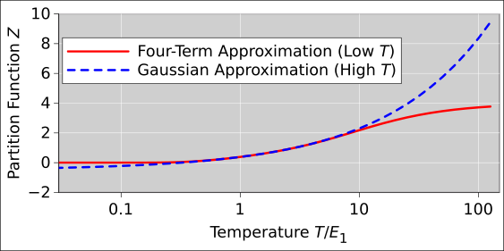
At low temperatures, we can approximate equation 26.32 by grinding out the first few terms of the sum. That gives us a power series:
| (26.34) |
At high temperatures, we need a different approximation:
| (26.35) |
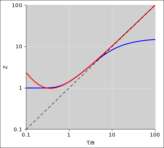
At high enough temperatures, the partition function converges to T/θr. This asymptote is shown by the dashed line in figure 26.2.
The low-temperature approximation is shown by the blue curve in figure 26.2. It is good for all T/θr ≤ 2.
The high-temperature approximation is shown by the red curve in figure 26.2. It is good for all T/θr ≥ 2.
We can rewrite the high-temperature limit in an interesting form:
| (26.36) |
where rg is the radius of gyration, defined as rg2 := Icirc/m∘. This is a well-known quantity in mechanics. It is a measure of the “effective” size of the rotor. The thermal de Broglie length λ is defined in equation 26.2.
It is interesting to contrast equation 26.1 with equation 26.35. Both involve the thermal de Broglie length, λ. However, the former compares λ to the size of the box, while the latter compares λ to the size of the molecule – quite independent of the size of the box.
Scaling arguments are always fun. Let’s see what happens when we scale a box containing an ideal gas. We restrict attention to a tabletop nonrelativistic monatomic nondegenerate ideal gas in three dimensions except where otherwise stated). In particular, in this section we do not consider the rotational degrees of freedom mentioned in section 26.3.
Consider the case where our gas starts out in a three-dimensional box of volume V. Then we increase each of the linear dimensions by a factor of α. Then the volume increases by a factor of α3. The energy of each microstate decreases by a factor of α2 in accordance with the usual nonrelativistic kinetic energy formula p2/(2m) where p = ℏk. (Because the gas is monatomic and ideal, this kinetic energy is the total energy.)
This is interesting because if we also scale β by a factor of α2, then every term in equation 26.69 is left unchanged, i.e. every term scales like the zeroth power of α. That implies that the partition function itself is unchanged, which in turn implies that the entropy is unchanged. We can summarize this as:
| (26.37) |
where the RHS of this equation is some as-yet-unknown function of entropy, but is not a function of β or V. (We continue to assume constant N, i.e. constant number of particles.)
Equation 26.37 is useful in a number of ways. For starters, we can use it to eliminate temperature in favor of entropy in equation 26.10. Plugging in, we get
| E = |
|
| (26.38) |
That’s useful because pressure is defined as a derivative of the energy at constant entropy in accordance with equation 7.6. Applying the definition to the present case, we get
| (26.39) |
Plugging the last line of equation 26.39 into equation 26.10, we find
| (26.40) |
which is the celebrated ideal gas law. It is quite useful. However, it is not, by itself, a complete description of the ideal gas; we need another equation (such as equation 26.37) to get a reasonably complete picture. All this can be derived from the partition function, subject to suitable restrictions.
It is worthwhile to use equation 26.40 to eliminate the β dependence from equation 26.37. That gives us, after some rearranging,
| (26.41) |
See equation 26.45 for a more general expression.
In this section we generalize the results of section 26.4 to cover polyatomic gases. We continue to restrict attention to a tabletop nonrelativistic nondegenerate ideal gas in three dimensions ... except where otherwise stated.
We need to be careful, because the energy-versus-temperature relationship will no longer be given by equation 26.10. That equation only accounts for the kinetic energy of the gas particles, whereas the polyatomic gas will have rotational and vibrational modes that make additional contributions to the energy.
We now hypothesize that the energy in these additional modes will scale in proportion to the kinetic energy, at least approximately. This hypothesis seems somewhat plausible, since we have seen that the total energy of a particle in a box is proportional to temperature, and the total energy of a harmonic oscillator is proportional to temperature except at the very lowest temperatures. So if it turns out that other things are also proportional to temperature, we won’t be too surprised. On the other hand, a plausible hypothesis is not at all the same as a proof, and we shall see that the total energy is not always proportional to temperature.
To make progress, we say that any gas that upholds equation 26.42, where the RHS is constant, or at worst a slowly-varying function of temperature, is (by definition) a polytropic gas.
| (26.42) |
We write the RHS as a peculiar function of γ in accordance with tradition, and to simplify results such as equation 26.50. There are lots of physical systems that more-or-less fit this pattern. In particular, given a system of N particles, each with D▯ quadratic degrees of freedom, equipartition tells us that
| (26.43) |
as discussed in section 25.2. Of course, not everything is quadratic, so equation 26.42 is more general than equation 26.43.
When non-quadratic degrees of freedom can be ignored, we can write:
| (26.44) |
You can see that γ = 5/3 for a monatomic gas in three dimensions. See table 26.1 for other examples. Because of its role in equation 26.50, γ is conventionally called the ratio of specific heats. This same quantity γ is also called the adiabatic exponent, because of its role in equation 26.45. It is also very commonly called simply the “gamma” of the gas, since it is almost universally denoted by the symbol γ.
Using the same sort of arguments used in section 26.4, we find that equation 26.37 still holds, since it the main requirement is a total energy that scales like α−2.
Continuing down the same road, we find:
| (26.45) |
Some typical values for γ are given in table 26.1. As we shall see, theory predicts γ = 5/3 for a monatomic nonrelativistic nondegenerate ideal gas in three dimensions. For polyatomic gases, the gamma will be less. This is related to the number of “quadratic degrees of freedom” as discussed in section 26.7.
Gas θr/K T/K γ 2/(γ−1) He 293.15 1.66 3 H2 85.3 92.15 1.597 3.35 .. .. 293.15 1.41 4.87 N2 2.88 293.15 1.4 5 O2 2.07 293.15 1.4 5 Dry air 273.15 1.403 4.96 .. 293.15 1.402 4.98 .. 373.15 1.401 4.99 .. 473.15 1.398 5.03 .. 673.15 1.393 5.09 .. 1273.15 1.365 5.48 .. 2273.15 1.088 22.7 CO 2.77 293.15 1.4 5 Cl2 .351 293.15 1.34 5.88 H2O 293.15 1.33 6 CO2 293.15 1.30 6.66 Table 26.1: Values of θr and γ for common gases
Terminology: We define a polytropic process (not to be confused with polytropic gas) as any process that follows a law of the form PVn = c, This includes but is not limited to the case where the exponent n is the adiabatic exponent γ. Interesting cases include
Let’s calculate the energy content of a polytropic gas. Specifically, we calculate the amount of energy you could extract by letting the gas push against a piston as it expands isentropically from volume V to infinity, as you can confirm by doing the integral of PdV:
| (26.46) |
This means the ideal gas law (equation 26.40) can be extended to say:
| (26.47) |
This is interesting because PV has the dimensions of energy, and it is a common mistake to think of it as “the” energy of the gas. However we see from equation 26.47 and table 26.1 that PV is only 66% of the energy for helium, and only 40% of the energy for air.
You shouldn’t ask where the “missing” energy went. There is no missing energy here. There was never a valid reason to think that PV was “the” energy. The integral of PdV has the same dimensions as PV, but is not equal to PV. There’s more to physics than dimensional analysis.
Let’s calculate the heat capacities for a polytropic ideal gas. We retrace the steps used in section 26.2. Rather than starting from equation 26.10 to derive equation 26.11 and equation 26.11, we now start from equation 26.47 to derive the following for constant volume:
| (26.48) |
And similarly, for constant pressure:
| (26.49) |
The ratio of specific heats is
| (26.50) |
This is why γ deserves the name “ratio of specific heats” or “specific heat ratio”.
We can use equation 26.48 and equation 26.49 to get a useful expression for the entropy of a polytropic gas. We invoke the general definition of heat capacity – aka the entropy capacity, loosely speaking – namely equation 7.24.
| (26.51) |
We can integrate that along a contour of constant V to obtain:
| (26.52) |
where f() is some as-yet-unspecified function. As a check, note that for the ideal monatomic gas, γ = 5/3, so equation 26.52 has the same temperature-dependence as equation 26.18, as it should.
Similarly:
| (26.53) |
| (26.54) |
Let’s try to derive the entropy of a polytropic gas. We start by rewriting the partition function for a particle in a box (equation 26.1) as:
| (26.55) |
We then replace the 3 by
| (26.56) |
and turn the crank. As a generalization of equation 26.6 we have:
| (26.57) |
where L is some length I threw in to make the dimensions come out right.
Then in analogy to equation 26.13 we have
| (26.58) |
for some unspecified f(N). All of the temperature dependence is in the last term. You can check that this term is plausible, insofar as it agrees with equation 26.52. Similarly, all the volume dependence is in the next-to-last term. You can check that this is plausible, by considering an adiabatic process such that PVγ is constant, and PV=NkT. For such a process, equation 26.58 predicts zero change in entropy, as it should.
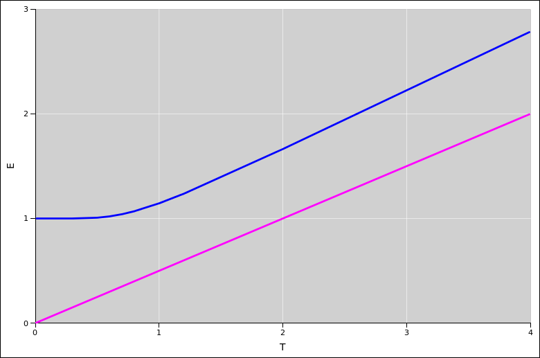
In this section we consider low temperatures, not just the high-temperature limit. For a single particle in a one-dimensional box, the partition function is given by equation 26.63. We calculate the energy from the partition function in the usual way, via equation 24.9.
Here the energy and temperature are measured in units of the ground-state energy (which depends on the size of the box). The blue curve shows the actual energy of the system; the magenta curve shows the high-temperature asymptote, namely E = 0.5 T.
The famous zero-point energy is clearly visible in this plot.
As you can see in the diagram, the slope of the E-versus-T curve starts out at zero and then increases. It actually becomes larger than 0.5. At higher temperatures (not shown in this diagram) it turns over, converging to 0.5 from above.
In this section we will temporarily lower our standards. We will do some things in the manner of “classical thermodynamics” i.e. the way they were done in the 19th century, before people knew about quantum mechanics.
Also in this section, we restrict attention to ideal gases, so that PV=NkT. This is quite a good approximation for typical gases under ordinary table-top conditions. We further assume that the gas is non-relativistic.
We now attempt to apply the pedestrian notion of equipartition, as expressed by equation 25.7. It tells us that for a classical system at temperature T, there is ½kT of energy (on average) for each quadratic degree of freedom. In particular, if there are N particles in the system and D▯ classical quadratic degrees of freedom per particle, the energy of the system is:
| (26.59) |
We assert that a box of monatomic gas has D▯=3 quadratic degrees of freedom per atom. That is, each atom is free to move in the X, Y, and Z directions, but has no other degrees of freedom that contribute to the average energy. (To understand why the potential energy does not contribute, see section 25.3.) This means that equation 26.59 is consistent with equation 26.10. However, remember that equation 26.10 was carefully calculated, based on little more than the energy-versus-momentum relationship for a free particle ... whereas equation 26.59 is based on a number of bold assumptions.
Things get more interesting when we assert that for a small linear molecule such as N2 or CO, there are D▯=5 degrees of freedom. The story here is that in addition to the aforementioned freedom to move in the X, Y, and Z directions, the molecule is also free to rotate in two directions. We assert that the molecule is not able to rotate around its axis of symmetry, because that degree of freedom is frozen out ... but it is free to tumble around two independent axes perpendicular to the axis of symmetry.
Going back to equation 26.59 and comparing it to equation 26.47, we find the two expressions are equivalent if and only if
| (26.60) |
You can now appreciate why the rightmost column of table 26.1 tabulates the quantity 2/(γ−1). The hope is that an experimental measurement of γ for some gas might tell us how many classical quadratic degrees of freedom there are for each particle in the gas, by means of the formula D▯=2/(γ−1). This hope is obviously unfulfilled in cases where formula gives a non-integer result. However, there are quite a few cases where we do get an integer result. This is understandable, because some of the degrees of freedom are not classical. In particular the “continuum energy” approximation is not valid. When the spacing between energy levels is comparable to kT, that degree of freedom is partiall frozen out and partially not. For details on this, see chapter 25.
You have to be a little bit careful even when 2/(γ−1) is an integer. For instance, as you might guess from table 26.1, there is a point near T=160K where the γ of molecular hydrogen passes through the value γ=1.5, corresponding to D▯=4, but this is absolutely not because hydrogen has four degrees of freedom. There are more than four degrees of freedom, but some of them are partially frozen out, and it is merely fortuitous if/when γ comes out to be an integer.
The γ values for Cl2 and CO2 are lower than you would expect for small linear molecules. This is because vibrational degrees of freedom are starting to come into play.
For an even more spectacular example of where classical ideas break down, including the idea of “degrees of freedom”, and the idea of “equipartition of energy” (i.e. 1/2 kT of energy per degree of freedom), look at the two-state system discussed in section 24.4.
Except for section 26.7, we derived everything we needed more-or-less from first principles: We used quantum mechanics to enumerate the microstates (figure 26.4), we calculated the microstate energy as p2/(2m), then constructed the partition function. The rest was just turning the crank, since there are well-known formulas for calculating the thermodynamic observables (energy, entropy, pressure, et cetera) in terms of the partition function.
This section shows how to derive the canonical partition function for a single particle in a box.
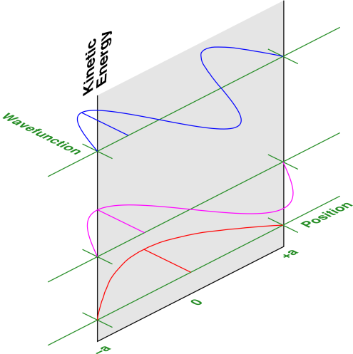
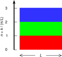
The three lowest-lying energy eigenstates for a one-dimensional particle in a box are illustrated in figure 26.4.
The wavevector of the nth state is denoted kn, and can be determined as follows: Observe that the ground-state wavefunction (n=1) picks up π (not 2π) units of phase from one end of the box to the other, and the nth state has n times as many wiggles as the ground state. That is,
| kn L = n π (26.61) |
where L is the length of the box.
As always, the momentum is p = ℏ k, so for a non-relativistic particle the the energy of the nth state is
| (26.62) |
and the partition function is therefore
| (26.63) |
where (as always) Λ denotes the thermal de Broglie length (equation 26.2), and where the first term in the partition function is:
| (26.64) |
and conversely
| (26.65) |
where E1 and p1 are the kinetic energy and the momentum of the n=1 state of the particle in a box.
In the low temperature limit, X is small, so only the first few terms are important in the sum on the RHS of equation 26.63. When X is less than 0.5, we can approximate Z to better than 1ppm accuracy as:
| (26.66) |
The probability of occupation of the two lowest-lying states are then:
| (26.67) |
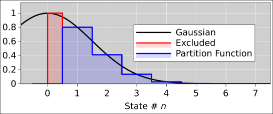
We now move away from the low temperature limit consider moderate and high temperatures. In this case, the sum in equation 26.63 can be approximated by an integral, to high accuracy.1
The integral is in fact a Gaussian integral, which makes things easy for us, since Gaussian integrals show up quite often in physics, and there are routine procedures for handling them. (See reference 56 for a review.) In fact, you can almost do this integral in your head, by making a scaling argument. The summand in equation 26.63 (which is also our integrand) is a Gaussian with a peak height essentially equal to unity, and with a width (along the n axis) that scales like L/Λ. So the area under the curve scales like L/Λ. If you do the math, the factors of 2 and factors of π drop out and you find that the area of a half-Gaussian is just L/Λ.
Figure 26.5 shows why we care about only half of the Gaussian. Also, if we want the area under the Gaussian curve to be a good approximation, it pays to account for the red shaded region that does not contribute to the partition function. Most textbooks overlook this, but it makes a dramatic improvement at the low end of the temperature range. Equation 26.68 gives much better than 1ppm accuracy all the way down to X=.5, where it mates up with equation 26.66 as shown in figure 26.6.
| (26.68) |
At sufficiently high temperature and/or low density, you can drop the 1/2.
We can use the partition function to derive anything we need to know about the thermodynamics of a particle in a box.
Let us now pass from one dimension to three dimensions. The partition function for a particle in a three-dimensional box can be derived using the same methods that led to equation 26.68. We won’t bother to display all the steps here. The exact expression for Z can be written in various ways, including:
| (26.69) |
In the high-temperature limit this reduces to:
| Z = |
| (26.70) |
where V is the volume of the box. The relationship between equation 26.68 and equation 26.70 is well-nigh unforgettable, based on dimensional analysis.
It turns out that Planck used h in connection with thermodynamics many years before anything resembling modern quantum mechanics was invented. Thermodynamics did not inherit h from quantum mechanics; it was actually the other way around. More importantly, you shouldn’t imagine that there is any dividing line between thermodynamics and quantum mechanics anyway. All the branches of physics are highly interconnected.
If we (temporarily) confine attention to the positive k axis, for a particle in a box, equation 26.61 the wavenumber of the nth basis state is kn = nπ/L. The momentum is therefore pn = ℏkn = nπℏ/L. Therefore, the spacing between states (along the the positive momentum axis) is πℏ/L. Meanwhile, there is no spacing along the position axis; the particle is within the box, but cannot be localized any more precisely than that. Therefore each state is (temporarily) associated with an area in phase space of πℏ or equivalently h/2. The states themselves do not have any extent in the p direction; area in phase space is the area between two states, the area bounded by the states.
For a particle in a box, running-wave states are not a solution to the equation of motion. Therefore, when we consider the k axis as a whole, we find that the area between one state and the next consists of two patches of area, one at positive k and another at negative k. Both values of k, positive and negative, correspond to the same physical state. Taking these two contributions together, the actual area per state is simply h.
Figure 26.7 shows the phase space for a particle in a box, with the lowest three areas color-coded. The area “associated” with a state is the area between that state and the preceding one.
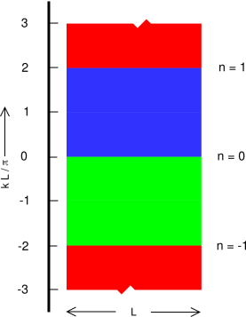
We now consider a particle subject to periodic boundary conditions with period L. This is analogous to water in a circular trough with circumference L. Running-wave states are allowed. The calculation is nearly the same as for a particle in a box, except that the wavenumber of the nth basis state is kn = 2nπ/L, which differs by a factor of 2 from the particle-in-a-box expression. Also, there is a n=0 state that we didn’t have in the box.
In this case, positive k corresponds to a rightward running wave, while negative k corresponds to a leftward running wave. These states are physically distinct, so each state has only one patch of area in phase space. The area is 2πℏ or simply h.
Figure 26.8 shows the phase space for this case, with the three lowest-energy basis states color coded. This is much simpler than the particle-in-a-box case (figure 26.7).
Figure 26.9 shows the analogous situation for a harmonic oscilator. Once again, the states themselves occupy zero area in phase space. When we talk about area in phase space, we talk about the area bounded between two states. In the figure, the states are represented by the boundary between one color and the next. The boundary has zero thickness.
For the harmonic oscillator (unlike a particle in a box) each state has nontrivial exent in the position-direction, not just the momentum-direction.
Any state of the system can be expressed as a linear combination of basis states. For example, if you want to create a state that is spatially localized somewhere within the box, this can be expressed as a linear combination of basis states.
Now it turns out that the process of taking linear combinations always preserve area in phase space. So each and every state, including any spatially-localized state, will occupy an area h in phase space. This fact is used in section 12.3.
Actually it has been known since the 1800s that any physically-realizable transformation preserves area in phase space; this is known as Liouville’s theorem. Any violation of this theorem would immediately violate many laws of physics, including the second law of thermodynamics, the Heisenberg uncertainty principle, the optical brightness theorem, the fluctuation/dissipation theorem, et cetera.