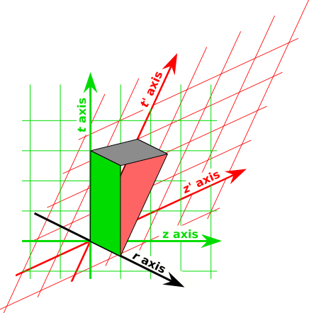
Figure 1: Electromagnetic Field Bivectors
Consider the following contrast:
| A beam of plain old electrons will repel another beam of plain old electrons. This is obvious in the frame comoving with the electrons, and what’s true in one frame must be true in all. | An electrically neutral wire carrying a current will attract another wire carrying current in the same direction. |
The repulsion of the charged beams is easily explained, as mentioned above.
Our task for today is to explain the attraction of the neutral wires. We could easily explain this using the conventional magnetic formulas ... but that would not tell us anything about the microscopic origins of magnetism. So as a starting point we will not use any facts about magnetism; instead that will be our goal and ending point. We shall see that the phenomenon we call magnetism must exist because of what we already know about electrostatics plus relativity. The so-called "magnetism" of an electromagnet is just a side effect of electrostatics in moving reference frames.
Electrostatics tells us that the electrons in one wire are strongly repelled by the electrons in the other wire. This is a huge effect, because the density of electrons in a piece of metal is huge (much larger than the density that could be achieved in an electron beam). But to first order this huge repulsion is canceled because the electrons in one wire are attracted to the positive metal ions in the other wire. If no current were flowing, there would be (to an excellent approximation) no attraction between between the wires.
So we need to carefully examine what changes when the electrons are moving relative to the positive metal ions.
As discussed in reference 1, it is best to represent the electromagnetic field as a bivector. What is conventionally called an electric field, in a given frame, is just an electromagnetic field bivector that has one of its edges oriented in the timelike direction in that frame. Similarly, what is conventionally called a magnetic field is just an electromagnetic field bivector that has both of its edges in purely spacelike directions, in the given frame.
The electromagnetic field of the electrons in the wire is purely electrical in the frame comoving with the electrons. The electromagnetic field of the positive metal ions is purely electrical in the frame comoving with the metal. So the puzzle is, how can these two purely electrical fields combine to make a magnetic field?
We will analyze the field of one of the wires. The wire runs in the z direction, right-to-left in figure 1. The lab frame’s time axis t runs vertically in the picture. The radial direction r (radially outward from the wire) is perpendicular to t and z in real life, and appears to run across the figure at an angle because of perspective.
The electric field bivector of the positive metal ions is shown in green. Using the wedge product, as discussed in reference 1, we can say that the electric field is in the r ∧ t direction, and in fact it is proportional to (1/r) ∧ t.
The "primed" reference frame is comoving with the electrons. The electric field bivector of the electrons goes like (1/r) ∧ t′, shown in red. And it has a minus sign, because the electrons are negatively charged.
Observe that the t′ axis is tilted relative to the t axis by an angle proportional to the electrons’ speed (relative to the ions).
The total electromagnetic field is the superposition of these two contributions. Add the bivectors edge-to-edge just as you add vectors tip-to-tail, with due regard to sign. The resultant is shown in gray. It is in the r ∧ z direction, and in fact it goes like (1/r) ∧ z, with additional factors proportional to the density and speed of the carriers. The exact answer is (2/r) ∧ I, where I is the current, as discussed in reference 2.
Note that all three bivectors in the figure are frame-independent physical objects. Everybody in every frame agrees that they are what they are.
The way you get into trouble is if people in different frames start arguing about frame-dependent notions such as whether such-and-such bivector is purely electrical or purely magnetic. The "electric" and "magnetic" pieces are merely components of the real, physical electromagnetic bivector, and as always, the decomposition into components is frame-dependent (and irrelevant to the physics).
Pedagogical hint: It is difficult to sketch figure 1 on a chalkboard with sufficient detail and clarity that students can follow it. Even the simplest "3D visual aids" give better results: grab a couple of pieces of card-stock and hold them edge to edge at an acute angle as shown in the figure. One card represents the electromagnetic field bivector of the metal ions, the other represents the electromagnetic field of the electrons, and you can wave your hand over the "mouth" they form and identify it as the resultant, i.e. the magnetic field.
Homework puzzle: Suppose you have a wire that produces a field that is, in the lab frame, purely magnetic. Can you fly past the wire at some special speed such that the field thereof becomes purely electrical?
Huge hint: Convince yourself that X ∧ (X∼) is a relativistic invariant, for any physical object X. In the case where X=p, the momentum 4-vector, the invariant is just the mass squared. What happens when we apply this idea to F, the electromagnetic field bivector? What is F ∧ (F∼)? See reference 1.
In section 1 we calculated everything we needed to know by looking at the fields themselves.
However, there is a classic thought experiment that explains a few things directly in terms of the amount of electrical charge. This is not really the smart way of looking at things, so I don’t recommend spending too much time on this, especially when first learning about the subject. On the other hand, a master of the subject should be able to see things from multiple points of view.
| One selling point for this charge-based approach is that it would work even if we didn’t know much about the structure of the fields, in particular if we didn’t know that the field was a bivector. | One of the many limitations of this approach is that it only works in the DC limit. The clever, sophisticated approach would be to use the Liénard-Wiechert potentials, as discussed in reference 3. |
We start in the lab frame, where the wire is at rest, i.e. the positive metal ions are at rest, and the electrons are flowing along the wire. In this frame, the field is purely magnetic. We can measure the strength of the field using a test charge that moves through the field.
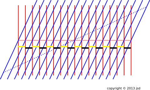
A spacetime diagram of this situation is shown in figure 2. The ion-core world-lines are shown in red, while the electron world-lines are shown in blue. The test charge is not shown.
We now restrict attention to the remarkable special case where the test charge is moving at the same speed as the electrons in the wire. This is probably completely impractical, but it makes for an interesting Gedankenexperiment.
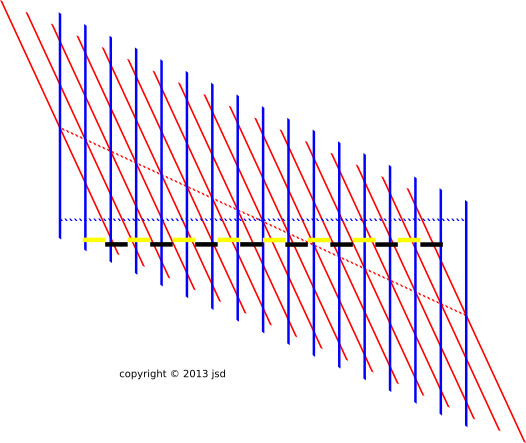
The next step is to view things in a frame comoving with the test charge (and with the electrons). This is shown in figure 3.
In this field, there is still a magnetic field, but it doesn’t affect the test charge, because the test charge is at rest.
As before, the test charge accelerates toward the wire, and this motion must be qualitatively the same in any frame. In this frame, the force must be entirely explained by an electric field, i.e. by the Coulomb interaction between charged particles.
Our understanding of this Coulomb interaction hinges on the definition of “density” as in charge density. This is a frame-dependent notion. To calculate the charge density in a particular frame, we count the amount of charge per unit length along a ruler at rest in that frame. Equivalently, we count the number of world-lines that cross a contour of constant t in the chosen frame.
In figure 2, we count the number of world-lines crossing yellow-and-black ruler. The horizontal spacing between red lines is the same as the horizontal spacing between blue lines. Indeed, there is one red line per unit length and one blue line per unit length.
In contrast, in figure 3, there is more than one red line per unit length, and less than one blue line per unit length. The wire has a net positive charge density. This is how we explain the force on the test charge, in this frame.
Again it must be emphasized that splitting the electromagntic field into an electric part and a magnetic part is not smart, and anything that focuses attention on a frame-dependent definition of density is not smart. Instead one should use the Liénard-Wiechert potentials, which permit a frame-independent calculation of the effect of source charge on a test charge. See reference 3.