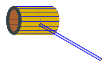
Figure 1: Field of a Long Straight Wire
The task for today is to calculate the electromagnetic field associated with the flow of current in a long straight wire. We choose to do this the modern way, representing the electromagnetic field as a bivector (not as a vector or pseudovector).
This allows us to understand Lenz’s law.
Note the contrast:
| We will make direct use of the modern form of the Maxwell equations, namely equation 1, as explained in reference 1. | We are not going to write the Maxwell equations in the old-fashioned way, in terms of cross products etc., and we are not going to represent the magnetic field as a vector (or pseudovector). |
This document is also available in PDF format. You may find this advantageous if your browser has trouble displaying standard HTML math symbols.
So, let’s begin. Clifford algebra allows us to write the so-called Maxwell equations as a single equation:
| ∇ F = |
| J (1) |
That equation can be shown to be entirely equivalent to the old-fashioned form of the Maxwell equations, as demonstrated in reference 1. That equation, along with the Lorentz force law, tell us everything we need to know about classical electromagnetism.
To analyze the wire, we make the following assumptions:
Therefore the current density is
| (2) |
Now we can plug this into the Maxwell equation(s) and turn the crank. We choose to use Clifford algebra ideas; an overview can be found in reference 3 and references therein. Additional useful references include reference 4, reference 5, and reference 6. For a discussion of the microscopic origins of the magnetic field, see reference 2.
We find it convenient to choose a set of basis vectors. We choose γ1 as the basis vector in the x direction, γ2 as the basis vector in the y direction, and γ3 as the basis vector in the z direction. These basis vectors are orthonormal. Nowhere do we assume that they form a right-handed set.
Using this basis, we can expand the ∇ operator in terms of its components, namely
| ∇ = γ1 (∂/∂x) + γ2 (∂/∂y) (3) |
where we have omitted the t and z derivatives because they vanish by symmetry.
We use the symbol I to denote the vector current. If you want the corresponding scalar, that is denoted Im, where the subscript m means “in the direction of the meter”. For simplicity, we hereby assume that the meter is oriented so that it measures current in the +z (not −z) direction, which means that
| (4) |
Let’s start by solving the equation inside the wire. We are looking for some F that has a constant derivative. We shouldn’t be too surprised if it is linear in the x and y coordinates, since the x-derivative of x is a constant and the y-derivative of y is a constant.
A good guess for F would be to write
| F = axγ1γ3 + byγ2γ3 + G (5) |
Where a and b are constants to be determined, G is any solution to the homogeneous equation ∇ F = 0. We will have more to say about G anon.
Plugging this into equation 1 we can find suitable values for a and b, with the result that the field inside the wire is
| F = |
|
| (x γ1γ3 + y γ2γ3) + G [inside] (6) |
Next, let’s consider what happens outside the wire. We shouldn’t be
too surprised if the field falls off in inverse proportion to the
distance from the axis. This is what we would expect based on a
Gauss’s law argument. Those who are not familiar with Gauss’s law can
verify that the following guess:
| F = |
|
| (x γ1γ3 + y γ2γ3) + G [outside] (7) |
is in fact a very good guess. It satisfies the Maxwell equation outside the wire (∇ F = 0) and also agrees with the other solution (equation 6) where they meet at the boundary of the wire (x2+y2 = Rw2).
At this point we will observe that G=0 produces a satisfactory solution for F. In fact, although we won’t prove it here, the solution is unique. Given the way we have chosen a and b, G=0 is the only G function that causes equation 7 to satisfy the boundary conditions (vanishing at large distances) and the required symmetries (independent of z, and rotationally invariant in the plane perpendicular to z) and is time-independent.
You should not, however, get into the habit of assuming that G=0 in problems of this sort. In this case G is zero only because we chose lucky values for a and b in equation 5. If we had instead chosen a′ = 2a and b′ = 0, then a nonzero G would have been necessary (and sufficient) to give us a satisfactory solution for F.
We can tidy up equation 7 quite a bit by writing it in a more vector-friendly basis-independent form, as follows:
We start by defining the position vector in all generality:
| r := xγ1 + yγ2 + zγ3 (8) |
The component of r parallel to I is given by the usual Gram-Schmidt formula:
| rI := I |
| (9) |
and you can verify that I · rI = I · r.
The component of r perpendicular to I is what’s left, namely, in all generality:
| r⊥:= r − rI (10) |
Applying these general definitions to our specific geometry, namely cylindrical coordinates with the axis in the γ3 direction, we find:
| (11) |
This r⊥ is the radius vector in cylindrical coordinates, always perpendicular to the z-axis. The square of its length is r⊥2 = x2+y2.
We also recall the definition of the I vector, equation 4. Putting the pieces together, we see that the field outside a long straight wire is
| (12) |
where we have used the fact that r⊥/r⊥2 is the reciprocal of r⊥, as you can verify by multiplying them together.
It might be even better to write this as
| (13) |
which is equivalent since by construction r⊥ is perpendicular to I.
The orientation of this field is shown by the blue rectangular bivectors in figure 1. Remember to write the field as (1/r⊥) ∧ I with the position vector first and the current vector second. This means that the edge of the field bivector that is closest to the wire is oriented opposite to the current. Lenz’s law is a useful reminder of this oppositeness, as discussed in section 5.
We can combine the expression for the field inside the wire and the field outside the wire as follows:
| F = |
|
| (14) |
It is very useful to notice that R (the radius of the wire) does not appear in the expressions for the field outside the wire. The only thing that matters is the total current, and the inverse distance from the center of the wire.
First, suppose we draw a circle in the XY plane, centered on the wire, as (for example) the red, dashed circle in figure 1. The circumference of this circle is 2πr⊥.
Next, note that we can rewrite equation 13 in the suggestive form:
| (15) |
and it is absolutely not a coincidence that 2πr⊥ occurs in both the expression for the circumference and the expression for the field.
In fact there is a very general mathematical theorem that goes as follows: For almost any F you can think of – including but not limited to the electromagnetic field F – ∇ ∧ F can be considered some sort of flow-density. Then, given any patch of surface S, the total flux of ∇ ∧ F flowing through the surface is equal to the line integral of F itself, integrated along the boundary of the surface. That is:
| ∫ |
| ∇ ∧ F = | ∫ |
| F (16) |
This is called Stokes’s Theorem. For the next level of detail, see reference 7.
As a corollary of this theorem, we can use equation 1 which gives us a nice expression for ∇F in terms of the current density. Plugging in, we obtain:
| ∫ |
| F = |
| IS (17) |
This is called Ampère’s Law. It says that the integral of the magnetic field (integrated around some loop ∂S) is equal to the current flowing through the area S bounded by the loop, with a factor of (1/є0c) thrown in to make the units come out right.
We have made use of the fact that this is a magnetostatics problem, so that ∇F equals ∇∧F.
The work we did in section 1 shows that this result is true for the special case of a circular loop around a long straight wire. Ampère’s Law is upheld everywhere outside and inside the wire, in accordance with equation 14.
With some additional geometrical arguments you can convince yourself that equation 16 must be true in general, for any shape of loop and for any distribution of current density; see reference 8.
In some sense, calculating the magnetic field by direct use of equation 1 is the hard way to do it … but we needed to do it that way once, in order to explain the origin of Ampère’s Law. However, now that we have Ampère’s Law, we can use it to our advantage. It makes equation 15 well-nigh unforgettable. The field is proportional to the current and inversely proportional to 2πr⊥ in accordance with the circumference of a circle via Stokes’s Theorem, and there is a factor of (1/є0c) inherited from the RHS of equation 1.
In section 3, we applied Stokes’s Theorem to the magnetic field. Now let’s apply it to the electric field.
We shall see that this leads to a simple yet exceedingly powerful corollary to the Maxwell equations:
| (18) |
which is pronounced “voltage equals flux dot”.
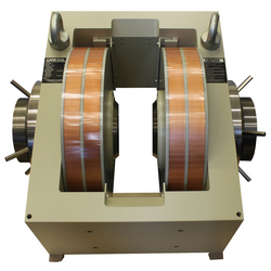
There is a wonderful hands-on demo that illustrates this. Start with a short piece of copper pipe, with fairly thick walls, made of OFHC copper. Attach a non-metallic handle as shown in figure 2. Soak it in liquid nitrogen to increase the electrical conductivity even more.
Put it into the high-field region of a big electromagnet. Let visitors wiggle it around. They will find that it is easy to move the pipe in the field so long as it remains in the same orientation. However, it is very hard to change the orientation by twisting the handle.
Using a fairly narrow handle provides mechanical disadvantage which makes the demo more effective.
This can be understood as follows: Because of the high conductivity, there cannot be much voltage drop around the circumference of the pipe. Therefore there cannot be any large quick change in the flux through the pipe. In the short term, the pipe is essentially a powerful bar magnet.
Because the electrical resistance is not quite zero, you can flip the pipe if you are persistent enough.
To summarize: In empty space, where there are no big chunks of copper, it is common to have changing magnetic fields, which are necessarily associated with electric field vectors chasing their tails around and around. In contrast, when there is a nearly perfectly conducting loop, we use the “voltage equals flux dot” law in reverse: Since there cannot be much votage drop, there cannot be any large quick change in the flux. Any attempt to change the flux will induce a huge current in the copper. The current produces a magnetic field that cancels out the attempted change. This is an example of Lenz’s law, as discussed in section 5.
The “voltage equals flux dot” law has thousands of other applications, qualitative as well as quantitative.
So, let’s see where the “voltage equals flux dot” law comes from.
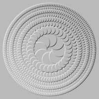
Suppose we have an electric field vector that chases its tail. It goes around and around in circles, as shown in figure 4. The strength of the field is proportional to the distance from the center.
The electric field here is obviously not the gradient of any potential. See reference 9.
This can be quantified by saying the electric part of the electromagnetic field bivector is something like this:
| (19) |
Now Stokes’s Theorem says that if we integrate that around a loop, that’s the same as integrating ∇∧FE over the area bounded by the loop.
Tangential remark: The loop doesn’t need to a physical wire or anything like that. An arbitrary imaginary loop will do. On the other hand, the voltage drop around the loop is particularly easy to measure if we string a wire along the loop.
All that doesn’t do us much good unless we can figure out what ∇∧FE is. That’s where Maxwell comes to the rescue. Equation 1 tells us that the only way F can have an electric piece like FE is if it also has a magnetic piece that looks like this:
| (20) |
The spacelike part of ∇ operating on F gives us
| (21) |
The timelike part of ∇ operating on F gives us
| (22) |
So we are called upon to find the integral over area of the time derivative of the magnetic field. If we move the derivative outside the integral, that’s just the time derivative of the magnetic flux.
So Stokes is telling us that the voltage drop around the loop is the time derivative of the flux threading the loop. Voltage equals flux dot.
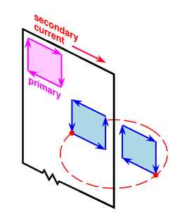
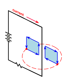
Instead of the battery shown in the previous figure, suppose that our wire loop is the secondary of a transformer. That is to say, we force some flux through the loop, as shown in magenta in the upper-left of the loop. The flux has the indicated orientation, and is increasing. In accordance with the Maxwell equation that says “voltage equals flux dot”, this induces a voltage drop around the loop, with the same orientation as the increasing flux. There is no minus sign in this law.
Using Ohm’s law or something similar, this produces a current in the direction of voltage drop around the loop, as shown by the red arrow. We call this the secondary current.
The current produces a field, namely the secondary field, with the orientation shown in blue. This secondary field necessarily has the opposite orientation to the change in primary flux.
This is one way of explaining Lenz’s law. The induced current produces a secondary field that opposes any change in the total flux through the loop.
This way of thinking about it depends on the fact that there is no minus sign in Ohm’s law. In other words, if you push on a charge, it diffuses in the direction of the force, not the opposite direction. By way of mnemonic, note that if the reverse were true, it would violate the second law of thermodynamics, since a resistor would produce useful energy out of nothing, rather than dissipating energy. A resistor across the terminals of a battery would serve to charge the battery, not discharge it
This qualitative version of Lenz’s law can be seen as a mathematical consequence of the Maxwell equations and Ohm’s law. It is useful as a mnemonic, to remind you of the oppositeness inherent in equation 13.
That way of thinking about it is not wrong, but Lenz’s law is actually deeper and more quantitative than that, as we can see from the following: Suppose the loop is a perfect conductor, i.e. zero resistance. Then the secondary field produces a flux equal and opposite to the change in the primary flux, so that the total flux through the loop remains constant for all time. We don’t need to worry about energy dissipation, because there isn’t any.
We see that rather than qualitatively “tending to oppose” the change in primary flux, the secondary flux is quantitatively equal and opposite. This is a direct consequence of the definition of perfect conductor. There can be no voltage around the loop, and therefore no flux dot. It’s just that simple.
For a conductor that is merely “almost” perfect, i.e. with a small but nonzero resistance, we need to talk about timescales. There will be an “L over R” time constant, where L is the inductance and R is the resistance. The induced current will keep the total change in flux at zero at short times. Then the induced current will die out on a timescale equal to L/R.
Remember that the wedge product of vectors is anticommutative, so you have to keep track of the order of the factors. To say the same thing the other way, if you write the factors in the other order it picks up a minus sign; for example, I ∧ (1/r⊥) = − I ∧ (1/r⊥). As previously mentioned, this means that the field produced by current in a wire has the following property: the edge of F nearest the wire is oriented opposite to the current.
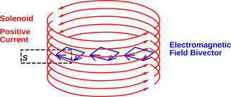
Another nice use of Ampère’s Law is to calculate the field inside a long solenoid. The situation is depicted in figure 6.
The electromagnetic field bivector F is purely magnetic, i.e. it is aligned in a purely spatial direction in spacetime, in the frame comoving with the solenoid. The bivector lies in the plane of symmetry, i.e. perpendicular to the axis of the solenoid. The field is uniform everywhere inside the solenoid, provided we don’t get too near the ends.
The orientation is such that if the current in the solenoid carries positive current circulating in one direction, the field bivector F circulates in the opposite direction.
The magnitude of the field F is:
| (23) |
where (I/L) is the current per unit length. The second line of the equation applies to the very common case where the circulating current is created by a wire carrying current Iw and there are N/L turns per unit length; each turn makes its own contribution to the total circulating current.
This result can be obtained in the familiar way, by applying Ampère’s Law to a surface A such as the one bounded by the black dashed line in figure 6.
All these results are based on equation 1. At no point have we found it necessary or even useful to calculate the old-fashioned magnetic field pseudovector. On the other hand, in the spirit of the correspondence principle, if you wish to compare equation 23 with the old-fashioned bivector expression, keep in mind that the magnetic component of F is, roughly speaking cB, not B.