The “big four” thermodynamic potentials are E, F, G, and H. That is:
| (15.1) |
Terminology note: Beware that H does not stand for Helmholtz (or for heat); H is the enthalpy. This is discussed in more detail in section 15.9.7.
There are systematic relationships between these quantities, as spelled out in section 15.7.
Depending on details of how the system is constrained, some one of these potentials might be useful for predicting equilibrium, stability, and spontaneity, as discussed in chapter 14.
Let’s establish a little bit of background. We will soon need to use the fact that
| d(P V) = PdV + VdP (15.2) |
which is just the rule for differentiating a product. For present purposes, we do not care about the physical significance of P and V; this is just math. This formula applies to any two variables (not just P and V), provided they were differentiable to begin with. Note that this rule is intimately related to the idea of integrating by parts, as you can see by writing it as
Note that the RHS of equation 15.3b could be obtained two ways, either by direct integration of the RHS of equation 15.3a, or by integrating the LHS, integrating by parts.
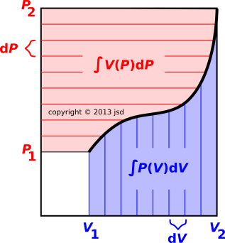
The idea behind integration by parts can be visualized using the indicator diagram in figure 15.1. The black dividing line represents the equation of state, showing P as a function of V (and vice versa). The blue-shaded region is the area under the curve, namely ∫PdV, where the P in the integrand is not any old P, but rather the P(V) you compute as a function of V, according the equation of state. By the same logic, the red-shaded region has area ∫VdP, by which we mean ∫V(P)dP, computing V(P) as function of P, according to the equation of state.
The large overall rectangle has height P2, width V2, and area P2 V2. The small unshaded rectangle has area P1 V1. So the entire shaded region has area Δ(PV). One way of looking at it is to say the area of any rectangle is ∫∫dPdV where here P and V range over the whole rectangle, without regard to the equation of state.
If you think of ∫PdV as the work, you can think of ∫VdP as the krow, i.e. the reverse work, i.e. the shaded area minus the work. Equivalently we can say that it is the entire area of the indicator diagram, minus the small unshaded rectangle, minus the work.
We can rewrite equation 15.3b as
| (15.4) |
which has the interesting property that the RHS depends only on the endpoints of the integration, independent of the details of the equation of state. This is in contrast to the LHS, where the work ∫PdV depends on the equation of state and the krow ∫ VdP also depends on the equation of state. If we hold the endpoints fixed and wiggle the equation of state, any wiggle that increases the work decreases the krow and vice versa.
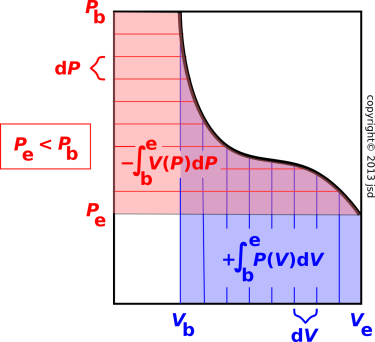
In the case where P happens to be a decreasing function of V, the picture looks different, but the bottom-line mathematical formula is the same and the meaning is the same.
Here subscript “b” stands for beginning, while subscript “e” stands for ending. The trick is to notice that the final pressure Pe is less than the initial pressure Pb, so the integral of V dP is negative. If we keep the endpoints the same and wiggle the equation of state, anything that makes the work ∫ P dV more positive makes the krow ∫ V dP more negative.
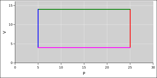
Consider the thermodynamic cycle shown on the indicator diagram in figure 15.3.
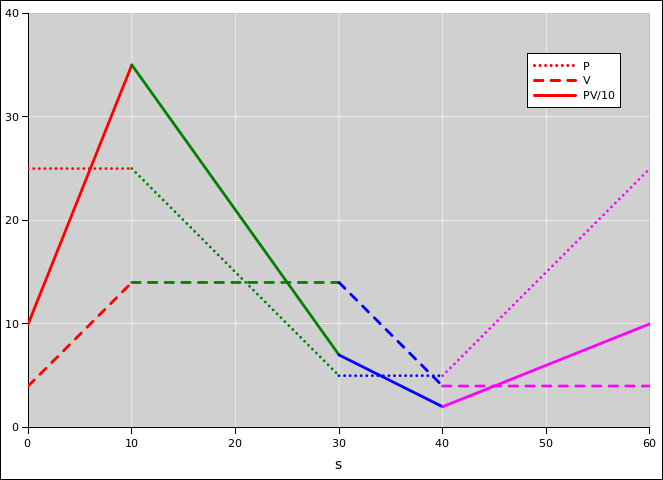
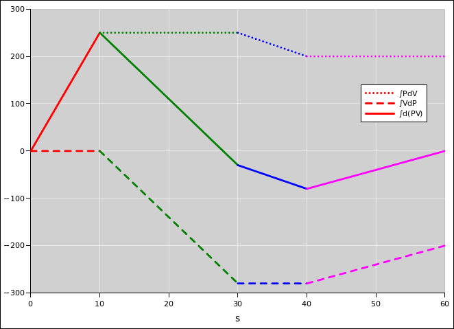
In figure 15.4, we plot P, V, and PV as functions of arc length s, as we go around the cycle, starting from the southeast corner. These are functions of state, so at the end of the cycle, they will certainly return to their initial values.
In figure 15.5, we plot some integrals. The integral of PdV is not a function of state; its value depends on the path whereby we reached the state. Ditto for the integral of VdP.
| Interestingly, the sum of ∫PdV plus ∫VdP is a function of state, because it is the integral of a gradient, namely the integral of d(PV). | In contrast, PdV is not the gradient of anything, and VdP is not the gradient of anything. See section 8.2 for details on this. |
You can verify that on a point-by-point basis, the ∫d(PV) curve is the algebraic sum of the other two curves.
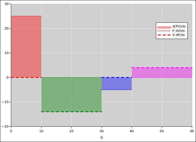
Figure 15.6 is another way of presenting the same basic idea. The shaded areas represent the derivative of PV.
In this section, in a departure from our usual practice, we are differentiating things with respect to the arc length s (rather than using the more sophisticated idea of gradient). This is not a good idea in general, but it is expedient in this special case. The whole notion of arc length is arbitrary and unphysical, because there is no natural notion of distance or angle in thermodynamic state space. If we rescaled the axes, it would have not the slightest effect on the real physics, it would change the arc length.
Because PV is a function of state, we know the area above the axis is equal to the area below the axis. When integrated over the whole cycle, the PdV contributions (red and blue) must be equal-and-opposite to the VdP contributions (green and magenta).
In other words, when we integrate over the whole cycle, we find that the total work is equal-and-opposite to the total krow. This applies to the whole cycle only; if we look at any particular leg of the cycle, or any other subset of the cycle, there is no reason to expect any simple relationship between the total work and the total krow. It is usually better to think in terms of the simple yet powerful local relationship between the derivatives: d(PV) = PdV + VdP.
The energy is one of the “big four” thermodynamic potentials.
The concept of energy has already been introduced; see chapter 1.
We hereby define the enthalpy as:
| H := E + P V (15.5) |
where H is the near-universally conventional symbol for enthalpy, E is the energy, V is the volume of the system, and P is the pressure on the system. We will briefly explore some of the mathematical consequences of this definition, and then explain what enthalpy is good for.
Differentiating equation 15.5 and using equation 7.8 and equation 15.2, we find that
| (15.6) |
which runs nearly parallel to equation 7.8; on the RHS we have transformed −PdV into VdP, and of course the LHS is enthalpy instead of energy.
This trick of transforming xdy into −ydx (with a leftover d(xy) term) is an example of a Legendre transformation. In general, the Legendre transformation is a very powerful tool with many applications, not limited to thermodynamics. See reference 44.
In the chemistry lab, it is common to carry out reactions under conditions of constant pressure. If the reaction causes the system to expand or contract, it will do work against the surroundings. This work will change the energy ... but it will not change the enthalpy, because dH depends on VdP, and dP is zero, since we assumed constant pressure.
This means that under conditions of constant pressure, it is often easier to keep track of the enthalpy than to keep track of the energy.
For simple reactions that take place in aqueous solution, usually both dP and dV are zero to a good approximation, and there is no advantage to using enthalpy instead of energy. In contrast, gas-phase reactions commonly involve a huge change in volume. Consider for example the decay of ozone: 2O3 → 3O2.
Enthalpy is important in fluid dynamics. For example, Bernoulli’s principle, which is often a convenient way to calculate the pressure, can be interpreted as a statement about the enthalpy of a parcel of fluid. It is often claimed to be a statement about energy, but this claim is bogus. The claim is plausible at the level of dimensional analysis, but that’s not good enough; there is more to physics than dimensional analysis.
See section 15.9 for an example of how enthalpy can be put to good use.
It is important to keep in mind that whenever we write something like H = E + PV, it is shorthand for
| (15.7) |
where every variable in this equation is a function of state, i.e. a function of the state of the stuff in the cell c. Specifically
It is important that these things be functions of state. This is an important issue of principle. The principle is sometimes obscured by the fact that
So, you might be tempted to write something like;
| (15.8) |
However, that is risky, and if you do something like that, it is up to you to demonstrate, on a case-by-case basis, that it is OK. Beware beware that there are lots of situations where it is not OK. For example:
It is informative to differentiate H with respect to P and S directly, using the chain rule. This gives us:
| dH = |
| ⎪ ⎪ ⎪ ⎪ |
| dP + |
| ⎪ ⎪ ⎪ ⎪ |
| dS (15.9) |
which is interesting because we can compare it, term by term, with equation 15.6. When we do that, we find that the following identities must hold:
| V = |
| ⎪ ⎪ ⎪ ⎪ |
| (15.10) |
and
| T = |
| ⎪ ⎪ ⎪ ⎪ |
| (15.11) |
which can be compared to our previous definition of temperature, equation 7.7, which says
| (15.12) |
(assuming the derivative exists). Equation 15.11 is not meant to redefine T; it is merely a useful corollary, based on of our earlier definition of T and our definition of H (equation 15.5).
In many situations – for instance when dealing with heat engines – it is convenient to keep track of the free energy of a given parcel. This is also known as the Helmholtz potential, or the Helmholtz free energy. It is defined as:
| F := E − T S (15.13) |
where F is the conventional symbol for free energy, E is (as always) the energy, S is the entropy, and T is the temperature of the parcel.
The free energy is extremely useful for analyzing the spontaneity and reversibility of transformations taking place at constant T and constant V. See chapter 14 for details.
See section 15.6 for a discussion of what is (or isn’t) “free” about the free energy.
The energy and the free energy are related to the partition function, as discussed in chapter 24.
Combining the ideas of section 15.3 and section 15.4, there are many situations where it is convenient to keep track of the free enthalpy. This is also known as the Gibbs potential or the Gibbs free enthalpy. It is defined as:
| (15.14) |
where G is the conventional symbol for free enthalpy. (Beware: G is all-too-commonly called the Gibbs free “energy” but that is a bit of a misnomer. Please call it the free enthalpy, to avoid confusion between F and G.)
The free enthalpy has many uses. For starters, it is extremely useful for analyzing the spontaneity and reversibility of transformations taking place at constant T and constant P, as discussed in chapter 14. (You should not however imagine that G is restricted to constant-T and/or constant-P situations, for reasons discussed in section 15.7.)
The notion of “available energy” content in a region is mostly a bad idea. It is an idea left over from cramped thermodynamics that does not generalize well to uncramped thermodynamics.
The notion of “free energy” is often misunderstood. Indeed the term “free energy” practically begs to be misunderstood.
It is superficially tempting to divide the energy E into two pieces, the “free” energy F and the “unfree” energy TS, but that’s just a pointless word-game as far as I can tell, with no connection to the ordinary meaning of “free” and with no connection to useful physics, except possibly in a few unusual situations.
To repeat: You should not imagine that the free energy is the “thermodynamically available” part of the energy. Similarly you should not imagine that TS is the “unavailable” part of the energy.
The free energy of a given parcel is a function of state, and in particular is a function of the thermodynamic state of that parcel. That is, for parcel #1 we have F1 = E1 − T1 S1 and for parcel #2 we have F2 = E2 − T2 S2.
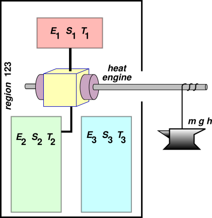
Suppose we hook up a heat engine as shown in figure 15.7. This is virtually the same as figure 1.2, except that here we imagine that there are two heat-sinks on the cold side, namely region #2 and region #3. Initially heat-sink #2 is in use, and heat-sink #3 is disconnected. We imagine that the heat-reservoir on the high side (region #1) is has much less heat capacity than either of the heat-sinks on the low side. Also, we have added an anvil so that the heat engine can do work against the gravitational field.
Assume the heat engine is maximally efficient. That is to say, it is reversible. Therefore its efficiency is the Carnot efficiency, (T1 − T2)/T2. We see that the amount of “thermodynamically available” energy depends on T2, whereas the free energy of parcel #1 does not. In particular, if T2 is cold enough, the work done by the heat engine will exceed the free energy of parcel #1. Indeed, in the limit that parcel #2 is very large and very cold (approaching absolute zero), the work done by the heat engine will converge to the entire energy E1, not the free energy F1.
We can underline this point by switching the cold-side connection from region #2 to region #3. This changes the amount of energy that we can get out of region #1, even though there has been no change in the state of region #1. This should prove beyond all doubt that “available energy” is not equal to the Helmholtz free energy F = E − TS. Similarly it is not equal to the Gibbs free enthalpy G = H − TS. It’s not even a function of state.
You may wish there were a definite state-function that would quantify the “available energy” of the gasoline, but wishing does not make it so.
We can reconcile the two previous itemized points by making the distinction between a scenario-function and a state-function. Something that is well defined in a careful scenario (involving two reservoirs and numerous restrictions) is not well defined for a single reservoir (all by itself with no restrictions).
Every minute spent learning about “available energy” is two minutes wasted, because everything you learn about it will have to be unlearned before you can do real, uncramped thermodynamics.
Constructive suggestion: In any case, if you find yourself trying to quantify the so-called “thermal energy” content of something, it is likely that you are asking the wrong question. Sometimes you can salvage part of the question by considering microscopic versus macroscopic forms of energy, but even this is risky. In most cases you will be much better off quantifying something else instead. As mentioned in section 17.1:
See chapter 19 for more on this.
In general, you should never assume you can figure out the nature of a thing merely by looking at the name of a thing. As discussed in reference 45, a titmouse is not a kind of mouse, and buckwheat is not a kind of wheat. As Voltaire remarked, the Holy Roman Empire was neither holy, nor Roman, nor an empire. By the same token, free energy is not the “free” part of the energy.
You are encouraged to skip this section. It exists primarily to dispel some misconceptions. However, experience indicates that discussing a misconception is almost as likely to consolidate the misconception as to dispel it. Your best option is to accept the idea that energy and entropy are primary and fundamental, whereas heat, work, and “available energy” are not. Accept the fact that any notion of “useful energy” belongs more to microeconomics than to physics.
Alas, some people stubbornly wish for there to be some state-function that tells us the “available energy”, and the purpose of this section is to disabuse them of that notion.
The plan is to analyze in more detail the system shown in figure 15.7. This provides a more-detailed proof of some of the assertions made in section 15.6.1.
The idea behind the calculation is that we start out with region 1 hotter than region 2. We operate the heat engine so as to raise the weight, doing work against gravity. This extracts energy and entropy from region 1. When T1 becomes equal to T2 we have extracted all of the energy that was available in this scenario, and the height of the weight tells us how much “available” energy we started with. We can then operate the heat engine in reverse, using it as a heat pump driven by the falling weight. We can arrange the direction of pumping so that energy and entropy are extracted from region 1, so that region 1 ends up colder than region 2, even though it started out warmer.
A major purpose here is to do everything in sufficient detail so that there is no doubt what we mean by the amount of energy “available” for doing work in this scenario. We measure the “available energy” quite simply and directly, by doing the work and measuring how much work is done. At any moment, the “available energy” is the amount of energy not (yet) transferred to the load.
This calculation is tantamount to rederiving the Carnot efficiency formula.
By conservation of energy we have:
| (15.15) |
Since the heat engine is reversible, we have:
| (15.16) |
Differentiating the energy, and using the fact that the reservoirs are held at constant volume, we have:
| (15.17) |
We assume that region 1 has a constant heat capacity over the range of interest. We assume that region 2 is an enormous heat bath, with an enormous heat capacity, and therefore a constant temperature.
| (15.18) |
Plugging equation 15.18 into equation 15.17 we obtain:
| (15.19) |
Doing some integrals gives us:
| (15.20) |
Remember: At any moment, the available energy is the energy that has not (yet) been transferred to the external load. Using conservation of energy (equation 15.15), we obtain:
| (15.21) |
Here’s the punchline: the RHS here is not the free energy F1 := E1 − T1 S1. It is “almost” of the right form, but it involves T2 instead of T1. It is provably not possible to write the available energy as F1 or F2 or F1 + F2 (except in the trivial case where T1 ≡ T2, in which case nobody is interested, because the available work is zero).
Equation 15.21 is a thinly-disguised variation of the Carnot efficiency formula. You should have known all along that the available energy could not be written as F1 or F2 or any linear combination of the two, because the Carnot efficiency formula depends on both T1 and T2, and it is nonlinear.
Here’s another way you should have known that the available energy cannot possible correspond to the free energy – without doing more than one line of calculation: Look at the definition F1 := E1 − T1 S1 and consider the asymptotic behavior. In the case of an ideal gas or anything else with a constant heat capacity, at high temperatures F must be negative. It must have a downward slope. Indeed it must be concave downward. Surely nobody thinks that a hot fluid has a negative available energy, or that the hotter it gets the less useful it is for driving a heat engine.
Thirdly and perhaps most importantly, we note again that we can change the amount of “available energy” by switching the lower side of the heat engine from heat-sink 2 to heat-sink 3. This changes the amount of work that the engine can do, without change the state of any of the reservoirs.
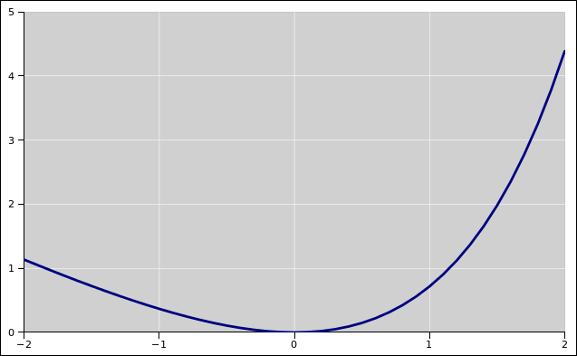
We now introduce ΔS to represent the amount of entropy transferred to region 1 from region 2 (via the heat engine), and we choose the constants such that ΔS is zero when the two regions are in equilibrium. That allows us to write the “available energy” as a simple function of ΔS:
| (15.22) |
This function is plotted in figure 15.8. You can see that the available energy is positive whenever region 1 is hotter or colder than region 2. It is usually more practical to store available energy in a region that is hotter than the heat sink, and you can understand why this is, because of the exponential in equation 15.22. However, at least in principle, anything that is colder than the heat sink also constitutes a source of available energy.
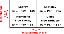
We have now encountered four quantities {E, F, G, H} all of which have dimensions of energy. The relationships among these quantities can be nicely summarized in two-dimensional charts, as in figure 15.9.
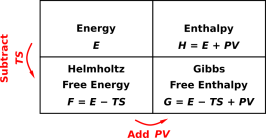
|
| |
| Figure 15.9: Energy, Enthalpy, Free Energy, and Free Enthalpy | Figure 15.10: Some Derivatives of E, F, G, and H | |
The four expressions in figure 15.10 constitute all of the expressions that can be generated by starting with equation 7.8 and applying Legendre transformations, without introducing any new variables. They are emphatically not the only valid ways of differentiating E, F, G, and H. Equation 7.12 is a very practical example – namely heat capacity – that does not show up in figure 15.10. It involves expressing dE in terms of dV and dT (rather than dV and dS). As another example, equation 26.10 naturally expresses the energy as a function of temperature, not as a function of entropy.
Beware: There is a widespread misconception that E is “naturally” (or necessarily) expressed in terms of V and S, while H is “naturally” (or necessarily) expressed in terms of P and S, and so on for F(V,T) and G(P,S). To get an idea of how widespread this misconception is, see reference 46 and references therein. Alas, there are no good reasons for such restrictions on the choice of variables.
These restrictions may be a crude attempt to solve the problems caused by taking shortcuts with the notation for partial derivatives. However, the restrictions are neither necessary nor sufficient to solve the problems. One key requirement for staying out of trouble is to always specify the direction when writing a partial derivative. That is, do not leave off the “at constant X” when writing the partial derivative at constant X. See section 7.5 and reference 3 for more on this.
Subject to some significant restrictions, you can derive a notion of conservation of enthalpy. Specifically, this is restricted to conditions of constant pressure, plus some additional technical restrictions. See chapter 14. (This stands in contrast to energy, which obeys a strict local conservation law without restrictions.) If the pressure is changing, the safest procedure is to keep track of the pressure and volume, apply the energy conservation law, and then calculate the enthalpy from the definition (equation 15.5) if desired.
Starting from equation 7.33 there is another whole family of Legendre transformations involving µN.
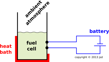
Consider the simplified fuel cell shown in figure 15.11.
Ideally, the fuel cell carries out the following reaction:
| (15.23) |
That equation is an OK place to start, but there’s a lot it isn’t telling us. For one thing, we have not yet begun to account for the energy and entropy.
There are four main energy reservoirs we need to keep track of:
| (15.24) |
The product on the RHS of equation 15.23 is a liquid, so, on a mole-for-mole basis, it takes up a lot less volume than the corresponding reactants. This means that as the reaction proceeds left-to-right, the collection of chemicals shrinks. In turn, that means that the ambient atmosphere does PdV work on the chemicals.
Also, although it’s not accounted for in equation 15.23 the way we have written it, the reaction must be balanced with respect to electrons (not just with respect to atoms). To make a long story short, this means that as the reaction proceeds, the chemicals do work against the battery.
Notation: The conventional symbols for electrical quantities include the charge Q and the voltage V. However, those letters mean something else in thermodynamics, so we are going to write the electrical work as F·dx. You can think of it as the force on the electrons times the distance the electrons move in the wire. Or you can imagine replacing the battery with a highly-efficient reversible motor, and measuring the genuine force and distance on the output shaft of the motor.
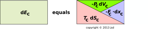
At this point we have enough variables to write down a useful expansion for the derivative of the energy:
| (15.25) |
For reasons that will be explained in a moment, it is useful to introduce the enthalpy H, and its gradient dH:
| (15.26) |
Plugging this into equation 15.25 we obtain
Equation 15.27b is predicated on the assumption that the pressure in our fuel cell (Pc) is constant all during the reaction, so that the derivative dPc vanishes.
Here’s one reason why it is worthwhile to analyze the system in terms of enthalpy: We can look at tabulated data to find the enthalpy of reaction for equation 15.23 (subject to mild restrictions). If the reaction is carried out under “standard conditions”, tables tell us the enthalpy of the chemicals Hc is 286 kJ/mol less on the RHS compared to the LHS. The enthalpy includes the energy of the reaction ΔE plus the PdV work (specifically ΔEc plus Pc dVc) ... neither of which we have evaluated separately. We could evaluate them, but there is no need to.
Tangential remark: Before we go on, let’s take another look at equation 15.25. From the point of view of mathematics, as well as fundamental physics, the PdV term and the F·dx term play exactly the same role. So the question arises, why do we include PdV in the definition of enthalpy ... but not F·dx???Partly it has to do with convention, but the convention is based on convenience. It is fairly common for the pressure to be constant, which makes it not very interesting, so we use the enthalpy formalism to make the uninteresting stuff drop out of the equation.
On the other hand, if you ever find yourself in a situation where there is an uninteresting F·dx term, you are encouraged to define your own enthalpy-like state function that deals with F·x the same way enthalpy deals with PV.
To make progress, we need more information. We need to know the entropy. It turns out that the entropy is known for oxygen, hydrogen, and water under standard conditions. This can be found, to a sufficient approximation, by starting at some very low temperature and integrating the heat capacity. (This procedure overlooks a certain amount of spectator entropy, but that is not important for present purposes.) Tabulated data tells us that the entropy (under standard conditions) of the RHS of equation 15.23 is 164 J/K/mol lower compared to the LHS.
At this point we can calculate the maximum amount of energy that can be delivered to the battery. Re-arranging equation 15.27b we have
| (15.28) |
The large negative ΔH means that a large amount of F·dx work can be done on the battery, although the rather large negative ΔS interferes with this somewhat. At 20∘ C, the TdS term contributes about 47.96 J/mol in the unhelpful direction, so the best we can expect from our fuel cell is about 238 kJ/mol. That represents about 83% efficiency. The efficiency is less that 100% because a certain amount of “waste heat” is being dumped into the heat bath.
Note that the Carnot efficiency would be essentially zero under these conditions, because the highest temperature in the device is the same as the lowest temperature. So the fuel cell exceeds the Carnot efficiency, by an enormous margin. This does not violate any laws of physics, because the Carnot formula applies to heat engines, and the fuel cell is not a heat engine.
If we were to burn the hydrogen and oxygen in an ordinary flame, and then use the flame to operate a heat engine, it would hardly matter how efficient the engine was, how reversible the engine was, because the chemisty of combustion is grossly irreversible, and this would be the dominant inefficiency of the overall process. See section 15.9.5 for more discussion of combustion.
For reasons that will explained in a moment, it is useful to introduce the Gibbs free enthalpy:
| (15.29) |
Plugging into equation 15.27b we obtain
where the last line is predicated on the assumption of constant temperature.
You should recognize the tactic. If our fuel cell is operating at constant temperature, we can declare the TdS term “uninteresting” and make it go away. This is the same tactic we used to make the PdV term go away in section 15.9.2.
In favorable situations, this means we have an even easier time calculating the F·dx work done by the fuel cell. All we need to do is look up the tabulated number for the Gibbs free enthalpy of reaction, for the reaction of interest. (This number will of course depend on temperature and pressure, but if the reaction takes place under “standard” or well-known conditions, it is likely that tabulated date will be available.)
In this section, we have made a great many simplifying assumptions. Let’s try to be explicit about some of the most-important and least-obvious assumptions. Here is a partial list:
However, unless otherwise stated, we assume that the overall process is reversible. In particular, there are no contributions to dSc other than a reversible flows of entropy across the C/H boundary. In mathematical terms: dSh = − dSc.
Back in the bad old days, before fuel cells were invented, there was no way to carry out the reaction in such a way that equation 15.27b applied. Approximately the only thing you could do was plain old combusion. If we remove the electrical connections from the fuel cell, all that remains is combustion, and the relevant enthalpy equation reduces to:
Previously, when analyzing the fuel cell, we had essentially two equations in two unknows: We used entropy considerations (the second law) to determine how much energy was flowing from the cell into the heat bath (in the form of TdS heat), and then used energy conservation (the first law) to determine how much energy was flowing from the cell into the battery (in the form of F·dx work).
Now, with the electrical connections removed, we have a problem. We how have two equations in only one unknown, and the two equations are inconsistent. Something has to give.
To make a long story short, the only way we can restore consistency is to stop assuming that the process is reversible. The laws of thermodynamics are telling us that if our heat bath is at some ordinary reasonable temperature, any attempt to use combustion of H2 in O2 to deliver energy to the heat bath will be grossly irreversible.
We now have a two-step process: We use the first law to determine how much energy will be delivered to the heat bath. We then create from scratch enough entropy so that this energy can be delivered in the form of TdS heat. This newly-created entropy is a new variable. We have returned to having two equations in two unknowns. This allows us to satisfy the second law while still satisfying the first law.
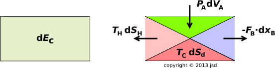
Let’s analyze this situation in more detail, using pictures. We start with figure 15.12, which is a pictorial representation of xsequation 15.25. This remains a valid equation.
Neither equation 15.25 nor figure 15.12 expresses conservation of energy. Indeed, they don’t express very much at all, beyond the assumption that E can be expressed as a differentiable function of three state-variables, namely S, x, and V.
It must be emphasized that each and every term in equation 15.25 is a function of state. Ditto for each and every term depicted in figure 15.12. The equation and the figure apply equally well to thermally-isolated and non-isolated systems. They apply equally well to reversible transformations and irreversible transformations.
Having said that, we can take two further steps: We assume that the heat flow across the A/H boundary is reversible. (This implies, among other things, that the cell and the heat bath are at the same temperature.) We then apply local conservation laws to each of the boundaries of the cell:
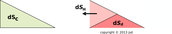
These three flows are diagrammed in figure 15.13.
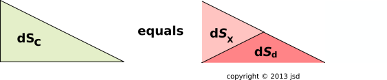
For a dissipative process, there is another term that must be included, in order to account for the possibility of entropy being created inside the cell. This term has got nothing to do with any flow. This is the Sd term in figure 15.15, and the corresponding TcdSd term in figure 15.13.
We have divided dS into two pieces:
To summarize:
In particular:
| For a reversible system, entropy is locally conserved, and of course energy is locally conserved. In such a system, each term on the RHS of equation 15.25 corresponds both to an internal change within the system and a flow across the boundary. | For an irreversible system, the dissipative part of dS is purely internal. It is not associated with any flow. It will not show up on any flow diagram. |
When we disconnected the fuel cell from the electrical load, the problem became overdetermined, and we had to add a new variable – the amount of dissipation – in order to make sense of the situation.
Now imagine that we keep the new variable and re-connect the electrical load. That makes the problem underdetermined. The amount of dissipation cannot be determined from the original statement of the problem, and without that, we cannot determine how much energy goes into the heat bath, or how much energy goes into the battery.
This is a correct representation of the actual physics.
As always, a good way to deal with an underdetermined problem is to obtain more information.
For example, if you think I2R losses are the dominant contribution to the dissipation, you can measure the current I and measure the resistivity of the electrolyte. The current of course depends on the rate of the reaction. This is not something you can determine by looking at the reaction equation (equation 15.23), but it is easy enough to measure.
If you slow down the reaction so that I2R losses are no longer dominant, you still have to worry about overvoltage issues, side reactions, and who-knows-what all else.
Consider the contrast:
| In equation 15.31b, the enthalpy could reasonably be identified as «the heat». However (!), examples of this kind are not enough to establish a general rule. | Our fuel cell is the poster child for illustrating that H is generally not the heat, as you can see in equation 15.27b for example. |
Conclusion: The enthapy is always the enthalpy, but it is not always equal to the heat.
Beware that all too often, documents that tabulate ΔH call it the «heat» of reaction, even though it really should be called the enthalpy of reaction.
More generally, it gets even worse than that. The term «heat» means different things to different people, depending on context. This includes, for example, the differential form TdS on the RHS of equation 15.31a. Other possibilities are discussed in section 17.1.