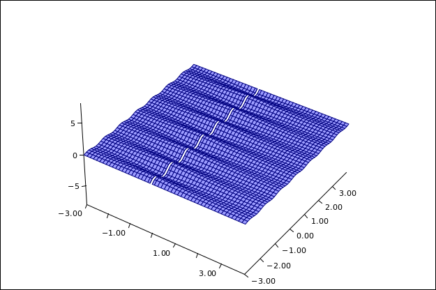
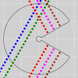
Figure 1: Orbits due to Curvature due to Darts
The notion of geodesic is an upgrade of our everday notion of straight line. Straight lines in particular and geodesics in general are fundamental and exceedingly important. In the first paragraph of the introduction to the Principia, Isaac Newton said:
“The description of right lines and circles, upon which geometry is founded, belongs to mechanics. Geometry does not teach us to draw these lines, but requires them to be drawn”.
The first law of motion says that a free particle moves in a straight line at a uniform speed. That’s true, but in order to make it useful, we need to be able to recognize straight paths and distinguish them from non-straight paths. (You could turn that around and use the motion of a free particle to “define” what we mean by a straight line, but it is simpler and far better to start with the geometrical idea of geodesic, and let that define what we mean by straight.)
Tangential remark: If you think about things in spacetime – that is, including the time dimension – then both parts of the first law of motion turn out to be exactly the same thing. The “straight line” part means there is a constant slope in the XY plane, while the “uniform speed” part means there is a constant slope in the XT plane. Considering all dimensions together, a uniform velocity is a straight line in spacetime, nothing more, nothing less. A discussion of this, along with an interactive diagram, can be found in reference 1.
Also, you have probably heard something about general relativity, including the idea that gravitation is explained by the “curvature” of spacetime. This document starts by explaining what we mean by a straight line in a curved space. It goes on to explain some of the important details about the direction in which the space is curved, how much it is curved, and how this produces the effects we call gravitation.
For a discussion of geodesics, shortest paths, straightest paths in a curved space, map projections, great circles, and rhumb lines, see reference 2.
It would be helpful to have some prior understanding of what we mean by spacetime, as discussed in reference 1 and elsewhere.
Here is a convenient way to correctly demonstrate the motion of a free particle in curved space. (This is almost but not quite a correct model of motion in spacetime.)
We use a two-dimensional surface as our model universe. To model the path of a particle, apply masking tape to this surface. For reasons explained in section 6, the tape will follow a geodesic (straight line) in the two-dimensional universe. Meanwhile, masking tape is so thin that it can bend as necessary in the third dimension (the embedding dimension). Be sure you use masking tape, which is designed to be non-stretchy (as opposed to something stretchy like electrical tape).
Lay out some tape and see what happens. Put down a couple of inches of tape to get things started, and then lay down the rest bit by bit. Let the tape guide itself, as discussed in section 2.2. As long as you don’t allow “crumpling” or “air pockets” under the tape, this process will automagically construct a nice straight geodesic, to an excellent approximation.
This stands in contrast to geometry in a curved space, which is non-Euclidean, as we shall see in a moment.
A cone is another shape that has extrinsic curvature but no intrinsic curvature (except at the singular point at the apex).
Observe that rolling the sheet into a cylinder or cone has no consequences for the geodesics; things that start out parallel remain parallel, et cetera. This is important because it shows that extrinsic curvature has no effect on the path of particles in our two-dimensional model world. That contrasts with intrinsic curvature, which will be demonstrated next.
If desired, you can make your own bowls out of cardboard. Slit the cardboard along one radius, form it into a shallow cone, and secure it with tape (inside and out) or with glue.
Lay out a geodesic that starts on the flat sheet and heads toward the bowl. When it reaches the bowl, it will refract.
Beware: Students might imagine that this is a model of the gravitational field of a planet, with the planet at the middle of the bowl, but it is not a good model of that. It is curved in the wrong direction. A much better model is presented in section 3.
And so on. You get the idea.
Note: Choose the color of the paper and the color of the bowls to contrast with the color of the tape. If you can get multiple colors of non-stretchy tape, so much the better.
Another suggestion: You can pile smaller bowls onto the back of the larger bowl, to change the shape of the potential.
Beware: Curvature has dimensions of inverse length. A large amount of curvature corresponds to a small radius of curvature. For non-experts who aren’t listening super-carefully, this can lead to communication problems (“Did you mean amount of curvature or radius of curvature?”). Sometimes it deteriorates into major conceptual confusion.
Remark: There is a familiar gravity that exists in the embedding world. Observe that this has no effect on the tape. Upward curvature affects the tape in exactly the same way as downward curvature. The models would work just the same upside-down, or in the weightless environment in a spaceship.
To repeat: The tape does not care whether the curvature is a bump or a pit. Consider what happens if you have a flat countertop with a bowl-shaped sink set into it. The tape runs straight along the countertop, but then drops down and follows the curvature of the inside of the sink. In all cases the geodesic will be bent toward the region of high intrinsic curvature.
A bump and a pit both have positive intrinsic curvature, as discussed in section 10.5. By way of contrast, a saddle has negative intrinsic curvature.
To construct geodesics, you want the tape to guide itself. Hold the supply of tape slightly slack; do not try to “force” the result to go in any particular direction. Instead put your finger on the most recently attached bit, then slide your finger forward, pressing the next bit into place.
To the extent possible, you want to avoid crumpling and stretching. (Also, of course, you want to avoid tearing.) If you are applying narrow tape to a gently-curving surface (such as a basketball) it should go down smoothly. On the other hand, if you try to apply wide tape to a sharply-curving surface (such as a marble) then crumpling is unavoidable and there is no point to the exercise. In intermediate cases, when there is a small amount of unavoidable crumpling, arrange it so that the middle of the tape is smooth and the two edges are equally crumpled. The idea is that the left and right edges of the tape define two nearby paths, and you want those two paths to have equal length.
Tangential discussion: By way of contrast, let us consider a model that is not a good model of motion in curved spacetime, but is often suggested, leading to tremendous confusion.
That is, imagine a marble rolling in a bowl. This can be contrasted with the tape-based model introduced in section 2.1.
| Rolling in a bowl more-or-less OK as a model of 17th-century classical physics, i.e. Newtonian gravitation. | Rolling in a bowl is a false and deceptive model of the modern physics, i.e. general relativity. |
| Rolling in a bowl depends on the fact that the bowl is embedded in the earth’s gravitational field. | The vastly superior tape-based model, as introduced in section 2.1, is independent of whatever gravity, if any, exists in the embedding world. |
If the shape of the bowl is just right – a paraboloid – the height of the bowl faithfully represents the classical gravitational potential. At each point, the slope of the bowl represents the gravitational field. (The fact that the marble rolls – rather than sliding freely – introduces some nonidealities, but let’s ignore that.)
If you use a glass bowl, you can demonstrate this to the whole room using an overhead projector.
To repeat: Although this models the classical physics to a fair approximation, it does not correctly model general relativity. In particular, the curvature of the bowl is not a good model of the spacetime curvature that general relativity uses to explain gravitation. Not at all.
There are several ways of seeing that it would be wrong to consider the bowl a model of general relativity.
To summarize: the alleged connection between “rolling in a bowl” and general relativity is essentially 100% wrong.
The model introduced in section 2.1 demonstrated the qualitative effects of curvature, but we have to refine it a bit if we want a really accurate model of, say, planetary orbits. It turns out that bowl-shaped potentials are not what we need. Not even close.
The world-line of a particle in orbit is best described as a helix. It goes around and around in two spacelike dimensions, while moving steadily forward in the timelike direction.
As pointed out by David Bowman, if you try to project that helix onto a two-dimensional model, there will be problems. Spacetime is curved (by gravity) in the timelike direction as well as the spacelike directions. So if you build a model that represents the two spacelike directions, suppressing the timelike direction, you can’t properly represent the sort of curvature that leads to planetary orbits.
We can do much better if we use our model to represent one timelike dimension and only one spacelike dimension. We will illustrate the gravitational field of a planet that exists for a long time (a long ways along the time axis). The gravitational field decreases as we move away from the planet in either direction along the X axis.
This can be modeled using darts, as shown in figure 1. The time axis runs vertically up the page, and the spacelike X axis runs horizontally across the page. The five ribs are made of two darts each, for a total of 10 darts. See section 11 for hints on how to fabricate darts.
I emphasize that the tape follows geodesics determined by the local curvature of spacetime at each point. Given an arrangement of darts, each trajectory is completely determined by its starting point and initial direction; there is no other choice involved.
Whenever the tape crosses a dart, the curvature of spacetime will deflect the trajectory toward the center. As it continues along, it will “orbit” the center, as you can see in the figure. In D=1+1, each trajectory looks like a sine-wave when viewed from above the page. One trajectory starts with an X value slightly left of center and completes a half-cycle before exiting at the top of the diagram. The next trajectory starts with an X value slightly right of center, and also completes a half-cycle. The third trajectory starts farther right of center, and completes only a small fraction of a cycle.
It is interesting to think about “what is the shortest path from point A1 to point A2”. The path in the presence of the darts is very different from what it would be in the absence of the darts. Actually in the presence of the darts (spacetime curvature) there are a couple of different geodesics that connect A1 to A2.
Hint: The stores around here sell masking tape that is 3/4” or 1” wide. Narrower tape is better for this demo. So you may want to divide the tape in half lengthwise. Do this while it was still on the roll, using a very sharp knife to cut through many layers.
If you attach the darts to a piece of acetate foil, you can set the whole thing on an overhead projector so everybody can see it. But letting people play with it hands-on is the best.
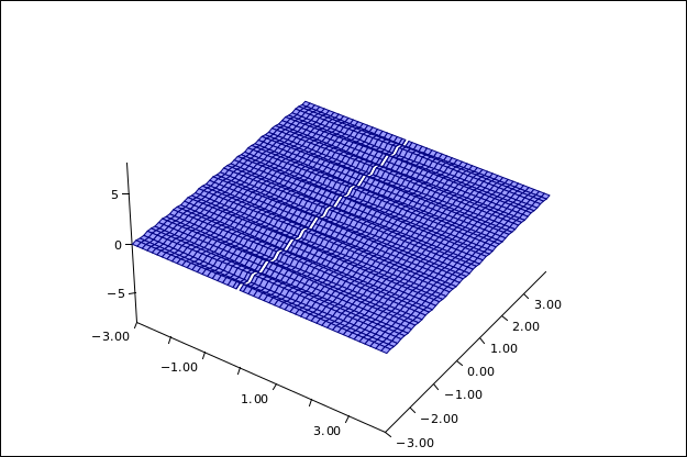
Figure 2 shows the same idea as figure 1. It shows the xt plane. The stripe along the contour of constant x=0 has no particular meaning; it just makes it easier to perceive the amplitude of the wiggles.
Figure 2 does not intersect the planet. It is a map of the xt plane at some nonzero y value, where y is big enough so that we don’t hit the planet.
This model is in some ways faithful to reality, and in some ways not.
You can improve the model by imagining a larger number of smaller wiggles, as in Figure 3. In your imagination, continue this process (an ever larger number of ever smaller wiggles) until there is curvature at all times, or close enough.
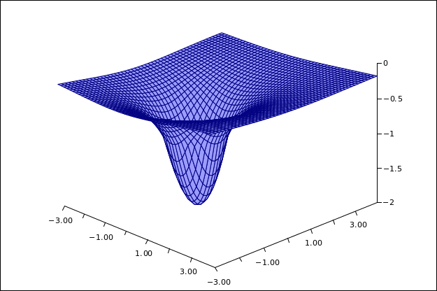
Diagrams such as figure 4 are very common, but not very faithful to the physics of general relativity. Such a diagram might result from a “trampoline” model, i.e. a heavy bowling ball resting on a trampoline, causing it to sag and stretch, forming a pit like the one shown in the diagram.
The bowling ball produces curvature in the membrane. So far so good. The problem arises when they try to model the dynamic by putting a marble in “orbit” around the bowling ball.
Alas, in the “pit” or “trampoline” model, none of the circles of constant radius are geodesics. If you tried to drive around such a circle, your inside tires would travel a shorter distance than your outside tires. That’s a problem, because a defining property of a geodesic is that if you drive along one, your left tires travel just as far as your right tires.
For a static gravitational field, the curvature that matters is the curvature in the timelike direction, as shown in figure 1 and figure 2.
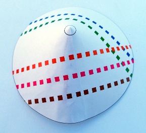
| Figure 6 shows some geodesics on a cone, viewed from above using an orthogonal projection. The geodesics are perfectly straight, even though this is not obvious in figure 5. | Things are easier to understand if we look at figure 5, which shows the exact same situation; however the cone has been split open and spread flat. Before flattening, the split has zero size; after flattening, it is 60∘ wide for the example we are discussing. |

|
| |
| Figure 5: Geodesics on a Cone – Orthogonal Projection | Figure 6: Geodesics on a Cone – Conformal Conic Projection | |
| The orthogonal projection may seem natural, but it is not perfect. Distances in the radial direction appear foreshortened, while distances in the azimuthal direction are unaffected, as discussed in section 4.3. This means we need to be careful about how we measure distances and angles. | Flattening makes the foreshortening problem go away. Although there is no such thing as a perfect projection from a curved space onto a flat space, a conformal conic projection of a cone comes pretty close; it is perfect except for things that cross the split. |
The large black circle has unit radius in cone-space, measured from the apex along the surface of the cone.
| It has less than unit radius when projected onto figure 5. This is an example of foreshortening. | It has unit radius, as it should, in figure 6. |
| In particular, the colored boxes in figure 5 are perfectly square in reality, even though they don’t look square in the diagram. If you measure things using the correct metric, you find that the box edges all have equal length, and the box diagonals all have equal length. | In figure 6, the square boxes look square, as they should. Distances and angles are just as they appear, except when things cross the split. |
Keep in mind that creatures living in the cone-world are completely unaffected by whatever projection (if any) we choose to use.
Note: When performing a conformal conic projection, you can split the cone along any radius; the choice doesn’t really matter. In figure 6 the split is at 3:00, but any other split would have served equally well to illustrate the interesting points, such as the fact that all the geodesics are straight. After all, the interesting physics is occurring on the original unsplit cone.
Here’s a riskier possibility: Rather than one split of size 60∘, you could have sixty splits of size 1∘, arranged evenly. This would be more symmetrical than figure 6. However, I’m not sure I recommend this, because it might create more misconceptions than it dispells. In particular, it would create the appearance of geodesics that gradually bend – but that’s only an appearance. In reality, geodesics (by definition!) do not bend.
In this section I used a computer to model the physics, but you can obtain the same results using a cardboard cone and masking tape.
It must be emphasized that the cone has zero intrinsic curvature, everywhere except at the apex. An ideal mathematical cone has infinite intrisinc curvature at the apex. However, infinities are hard to deal with properly, so let’s simplify the situation by grinding off the apex to form a smoothly-rounded region with small but nonzero size. All of the intrinsic curvature is confined to this region.
Note that our five geodesics do not enter the high-curvature region; they live entirely in the zero-curvature part of the cone.
In each of the diagrams, near the bottom we have five geodesics that are parallel. At the top, we have a group of two and also a group of three; members within each group are parallel to each other, but the two groups are not parallel. The difference beween the groups is that one passed to the left of the high-curvature region while the other passed to the right.
It is proverbial that parallel lines never meet. That is proverbially true, but not necessarily true! It only applies in a Euclidean space.
Here’s a simple counterexample: On a cylinder, there is no intrinsic curvature anywhere, but in special cases a straight line can meet itself, by circumnavigating the cylinder. You can see the back of your head, if you look in the right direction. Furthermore, in a flat space with periodic boundary conditions, you can see the back of your head if you look in any direction.
More generally, the whole notion of “parallel lines” breaks down in a non-Euclidean space. In figure 5, lines that start out parallel (near the bottom) wind up crossing (near the top) ... even though none of them actually experienced any curvature.
| Wrong way to think about it | Right way |
| Isn’t this some sort of spooky action at a distance? | No, it isn’t. |
| How can curvature “over there” cause the bending of a geodesic somewhere else? | It doesn’t. |
Keep in mind that geodesics do not bend – by definition. In figure 5, all five lines are straight. An observer living in the conical universe, moving along such a geodesic, would not experience any acceleration. Remember, in a non-Euclidean space, the whole idea of “parallel lines” breaks down. Lines that start out parallel don’t necessarily stay parallel ... even if they never visit any non-flat regions within the space.
Here’s another right way to think about it: To quantify the relationship between one geodesic and another, there is such a thing as the “equation of geodesic deviation”. The details are complicated, as discussed in section 12, but for present purposes it suffices to know that we have a differential equation that describes the relationship between nearby geodesics. If the geodesics are not sufficiently near to each other, i.e. if there is a gap between them, you can construct auxiliary geodesics in the gap, and then integrate across the gap. In figure 5, we can fill in the gap between the blue and green geodesics without difficulty. However, if we try to fill in the gap between the green and red geodesics, sooner or later one of the auxiliary geodesics will run into the high-curvature region. In this way we can understand the crossing of the green and red geodesics, without violating the principle that all of physics – including the idea of straightness itself – should be described in terms of what’s happening locally.
Similar remarks apply to figure 1; the darts create intrinsic curvature only at isolated points, i.e. the their tips and bases. The tapes in this example have been arranged so that they do not visit such points; they travel through parts of the space that have zero curvature.
Let’s choose polar coordinates in figure 6 to be (r, A) where r is the radius and A is the azimuthal angle. If we have one point at (r, A) and another at (r+δr, A+δA), then the square of the distance between them is:
| (1) |
For example, the length of the black arc in that figure is (5/6) 2πr, or simply (5/3)π, since it sits at r=1.
Similarly, let’s choose polar coordinates (ρ, α) in figure 5. Real physical distances in the azimuthal direction are just what they appear to be, namely δs = |ρ δα| (at constant ρ). For example, the black circle has length 2πρ, or simply (5/3)π, since it sits at ρ=5/6. Not coincidentally, this is the same length that we calculated in the previous paragraph. It’s the same physical length on the physical cardboard, after all.
However, the distances in the ρ direction are tricker. The projected radius ρ is shorter than the true physical distance – i.e. the slant length r – along the surface of the cone. Specifically:
| (2) |
where Θ is the opening angle of the cone, and f is the foreshortening factor, namely f :=sin(Θ/2). In our example f =5/6. So the metric in terms of the projected variables is:
| (3) |
In other words: Since the factor (1/f ) is greater than 1, true distances in the radial direction are larger than the projected diagram would lead you to believe. The fact that equation 3 includes a foreshortening factor in one term but not the other – so it is not just a scaled version of equation 1 – wreaks havoc with your intuition about distances and angles in the projected view.
You can create a real 3D paper cone, with preprinted geodesics, by printing out a suitable template and then cutting and gluing. Figure 7 shows an example. This provides “hands on” demonstrations of several interesting concepts about life in a non-Euclidean space, such as the fact that geodesics that start out parallel do not remain parallel, and may eventually cross, even though they are absolutely straight.
Reference 3 provides some .pdf files, similar to figure 6 but with additional features to help guide the assembly process.
Here are some suggestions for how to assemble the model:
(**) Cut close as you can to the ends of the black arcs. When assembled, these should meet end-to-end, with no gaps and no overlaps, to form circles. Other parts of the azimuthal cuts don’t need to be precise.
(**) However, cut close as you can to the ends of the black arcs.
It is almost as easy to apply glue to the “underlap” region. Put scratch paper under the work for the same reason as before, and then use another piece of scratch paper, with a straight edge, to mask the 2:00 azimuth, to keep glue from going where you don’t want it.
Using this technique, with a little bit of practice, you can make a nearly invisible joint.
The cone is a valuable pedagogical stepping stone, because even though it is a non-Euclidean space, it is as nearly Euclidean as it could possibly be. The cone has zero intrinsic curvature everywhere except at the apex. The only way for denizens of the cone-world to discover that their space is not completely flat is to do an experiment that somehow circumnavigates the apex.
| Put the model on the floor at your feet, or hang it on the wall at eye-height, so you can look at from a distance, looking directly along the axis of the cone. This should give you a pretty good approximation of an orthogonal projection. It should closely resemble figure 5. | Also take a closer look, with your line of sight perpendicular to some smallish region of the surface of the cone. In any such local region, the geodesics look straight, as in figure 7. Denizens of the cone-world are sure that the geodesics are straight, as they should be. |
The preprinted geodesics in the model are comparable to a combination of masking tape and measuring tape. That is, they are straight, with equally-spaced boxes along their length. Imagine some one-inch-wide tape decorated with one-inch squares all along its length.
It is important to learn the correct lessons from all this:
The fact that geodesics are sensitive to curvature elsewhere has direct application to astronomy and cosmology: You can measure the mass of a planet without ever setting foot on the surface. Just put a satellite in orbit around it, and apply Kepler’s laws. You can even measure the mass of a black hole this way, which is significant because the hole doesn’t have a surface that you could even imagine setting foot on.
Let us now discuss the physics of why masking tape can be used to construct straight lines.
For starters, masking tape has the wonderful property that it is supposed to be non-stretchy. You can verify this by trying to stretch a piece. (This stands in contrast to electrical tape, which is supposed to be stretch. If you have some stretchy tape, set it aside and get some non-stretchy tape.)
Secondly, note that it has definitely nonzero width. It is non-stretchy across its width, and also across innumerable diagonals, so it can hold itself straight, as discussed below.
Thirdly, the tape is very thin in the direction perpendicular to the width. This means it is easy to bend around an axis in the plane of the tape, even though it is orders of magnitude harder to bend around an axis perpendicular to the plane of the tape.
The size relationships can be summarized as:
| (4) |
This is significant, for the following reason: One thing you learn from Galileo’s book (or from analyzing the physics yourself) is that the stiffness of a bendable beam scales like the cube of the thickness in the plane of the bend. So if the tape is 100 times wider than it is thick, it is literally a million times more bendable in the direction it should bend (the XZ plane) than in the direction it shouldn’t (the XY plane).
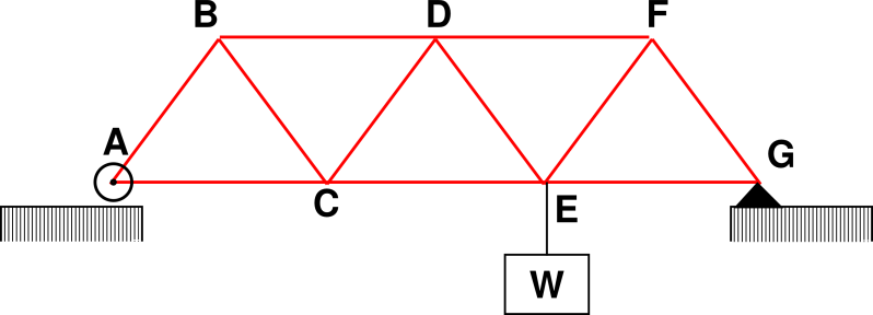
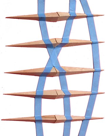
The tape holds itself rigid the same way a triangular truss holds itself rigid, as in the bridge in figure 8. If the strut-lengths don’t change, the overall shape of the structure cannot change.
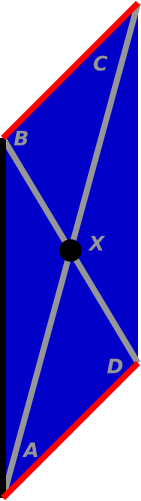
Figure 9 shows the kind of cross-bracing we are talking about. Lines drawn on the tape cannot stretch, and these define triangles that cannot change their shape. The length of line DB and line AC (shown in gray) cannot change, because the tape is non-stretchy. Similarly the length of line AD and line BC (shown in red) cannot change. In this way you can prove that all the triangles keep their shape. We know from high-school geometry that if the lengths stay the same, the angles must stay the same also. See reference 4 page 249 for a much more detailed and rigorous discussion.
You can mark triangles like this on your tape if you want, but you don’t have to. The tape keeps its shape even without the markings. The triangles are physically there, whether you mark them or not.
This notion of straightness, defined by cross-bracing, has numerous good properties. For one thing, if you stick an initial piece of tape to a surface, it defines a unique way of laying down the next piece, and then the next. This notion of straightness is reversible: You can trace the tape-path in the opposite direction and get the same result.
It is intriguing that in mathematics, lines are defined to be straight and have zero width, but in physics, if you want to make sure it is straight, it needs to have nonzero width (so the cross-braces have some leverage). You can pass to the limit of infinitesimal width, but not zero width.
| In your imagination, you can postulate straight lines and circles that exist in some formal, mathematical space. Such lines and circles are abstractions, devoid of physical meaning. | If you want to construct a “line” or anything else real life, making it straight requires physics, not just mathematics. |
Sometimes people try to “define” straightness by saying that a straight “line” is the shortest path between two points. That is, however, not the ideal definition. It would be better to say that any extremal path (either shortest or longest) is necessarily straight. You can show that the tape satisfies this definition, by the following argument: The two edges of the tape have equal length. The tape was manufactured to have that property, and it retains that property because it is non-stretchy. If you choose a hypothetical path that is not a geodesic – not straight – then nearby paths to one side will be slightly longer, and nearby paths to the other side will be slightly shorter. You cannot make the tape follow such a path without buckling.
Once we have a good way to make straight paths, it is a simple matter to create curved paths, by forcing one edge of the tape to follow a longer path than the other.
Tangential remark: Similar notions of curvature play a role in the expansion of the universe, as discussed in reference 5.
This is a bit of a digression, but it may be worth mentioning, because it is probably the simplest and easiest introduction to the idea of geodesics.
Start with an ordinary globe of the earth, preferably one with prominently marked lines of latitude and longitude. Stretch a string along the surface of the globe from point A to point B, where the points are not too close together.
We make use of the fact that in such a situation, the shortest path is also the straightest path. So a string under tension follows a geodesic. On a sphere, the geodesics are great-circle routes.
Note that the great-circle route from London to Los Angeles departs London on a northwesterly heading but approaches Los Angeles on a southwesterly heading. That is to say, it goes north for a while before going south. This looks perfectly normal when you see the string on the globe, but it would look mighty peculiar if plotted on a Mercator projection. The parallels of latitude are definitely not geodesics (except for the equator).
By way of background, suppose you travel from one point to another along some chosen path. You can use an odometer to measure the length of the path. This length will not usually be the same as the length of some other path. In particular, an odometer is not like a rigid ruler, which measures only one of the possible paths, namely the straight-line path.
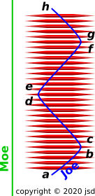
It turns out that ordinary clocks are more like odometers than like rulers. Suppose you travel along Joe’s path (shown in blue) in figure 10. The elapsed time along this path will not be the same as the elapsed time along Moe’s path (shown in green).
These two paths are different because Joe’s path has lots of curvature in the time direction. It is deeper in the gravitational potential.
One might be tempted to conclude that Joe’s clock (deep in the gravitational potential) will rack up more time than Moe’s clock (outside the potential). However, we have to be careful. When comparing clocks, we have to account for the breakdown of simultaneity at a distance. This is the same physics that explains the timing of the infamous traveling twins, as discussed in reference 6.
In this figure, the darts have a peculiar shape, with tapered ends separated by a non-tapered middle section. This produces a gravitational potential with sloping edges separated by a flat bottom section. This produces sharp turns (e.g. the [b, c] interval) separated by straight segments (e.g. the [c, d] interval). The purpose is to emphasize the analogy to the traveling twins.
If we look just at the length of the tape, Joe’s path is longer, because follows a crumpled path through spacetime. As a more precise way of arriving at the same conclusion, if we (temporarily!) look only at the straight sections of Joe’s path, Joe will think that Moe’s clocks are running relatively slowly, since Moe is moving relative to Joe. So Joe will think he is aging faster. However, Joe’s reference frame before point b is different from after point c. The idea of changing from one reference frame to another is explained in reference 6. It changes Joe’s notion of “same” time. This is the famous breakdown of simultaneity at a distance. This makes Joe see Moe as suddenly much older. The same thing happens in reverse during the [d, e] turnaround, only less so, because the distance between Moe and Joe is less, so the breakdown of simultaneity is less.
If you track down all the details, you find that as a general rule, a clock deeper in the gravitational potential racks up less time relative to a higher clock. This is the famous gravitational red shift.
You might be tempted to say that the deeper clock “runs slower” ... but you should resist this temptation. There is nothing wrong with either clock; both clocks run at the standard rate of 60 minutes per hour. The difference in elapsed time has nothing to do with the clocks. It has everything to do with the difference in path-length, and the breakdown of simultaneity at a distance. Clocks are like odometers. They measure the length (in the time direction) of the path. This very much depends on which path you choose.
This model shows the right general idea, but it is not exactly correct, because travel in spacelike directions makes a positive contribution to the overall spacetime interval, whereas travel in the timelike direction makes a negative contribution. The latter is hard to model.
Suppose you are helping a buddy with a plumbing project that involves cutting PVC pipes and gluing them into fittings. Your buddy sees no reason to buy a pipe cutter, since he has a perfectly good hacksaw. The problem is, if you want the joint to be strong, the pipe needs to be cut square, and this isn’t always easy to do. It’s not too hard under favorable conditions in the shop, but not so easy out in the field when the pipe is at a funny angle and there are other constraints.
The desired result can be obtained more easily and more reliably if the pipe is first properly marked ... then all you need to do is cut along the mark.
So now we come to the heart of the matter: What is the quick and easy way to create a “cut here” guide on the pipe?
Answer: Masking tape.
As discussed in previous sections, masking tape follows a geodesic. We assume the pipe is accurately cylindrical (otherwise the glue joint would fail anyway, so the whole exercise would be pointless). The geodesics of a cylinder are helices, including the zero-pitch helix which is a circle.
If you start the tape perpendicular to the axis of the pipe, the tape will come around and meet itself, making a zero-pitch helix, and you know you have succeeded. Cut parallel to the edge of the tape.
If you start the tape at an angle, it will come around and make a non-zero-pitch helix, and you know you need to re-do the taping.
This trick with the tape is super-accurate, super-quick, and super-easy.
The previous discussion has focused on what happens to a single point as it moves from place to place along a geodesic. In this section, we consider what happens to a vector as it moves from place to place along a geodesic. This is important, because it provides us with a particularly easy way to measure the curvature of the space.
Note the contrast:
| When we were just talking about position-space, at each position there was a point, and that’s all there was. | Now are talking about a vector field. That means at each point in position-space there is a vector space. We have a space of spaces. |
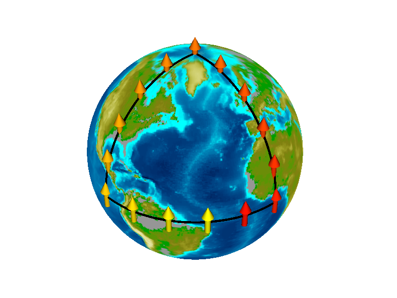
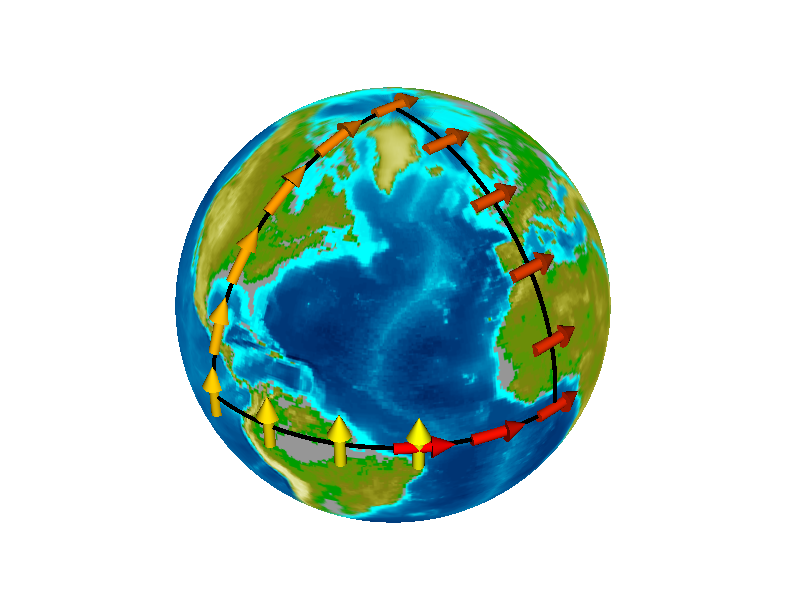
Consider the scenario shown in figure 11. We start with the yellow arrow that is located just north of the eastern tip of Brazil, on the equator at 45 degrees west longitude. The vector points due north. We then construct another vector 18 degrees farther west, at a point near the mouth of the Amazon. We take care that the new vector is parallel to the old vector. It also points due north. We keep constructing new vectors, each parallel to the previous one, until we come to 90 degrees west longitude, in the ocean south of Guatemala.
The next vector is constructed at a position due north of the previous one. We are now moving northward along a line of constant longitude, namely 90 degrees west longitude. All the arrows point toward the celestial north pole, i.e. a point high above the earth’s geographic north pole. As we move north, each of the arrows is parallel to the previous arrow.
In this context moving north means moving closer to the geographic north pole, following the surface of the earth (as opposed to moving directly closer to the celestial north pole, which would take us away from the surface). Note the contrast: We are using geographic north for the positioning, but we are comparing the orientation against celestial north.
We continue around the triangular path until we get back to the starting point. The final arrow appears to be parallel to the original arrow. There is nothing surprising about this.
Actually, due to general relativity, the final arrow is not quite exactly parallel to the original arrow, but the difference is far too small to be perceptible in figure 11. The rest of this section is devoted to explaining how it is possible for these two arrows to wind up not exactly parallel.
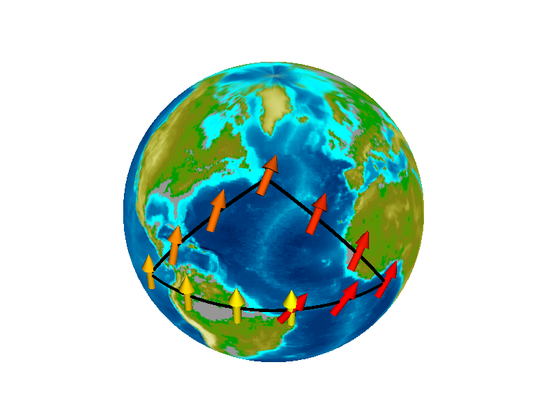
Consider the scenario shown in figure 12. It starts out exactly the same as the previous scenario. However, in this case we suppose that the arrows exist in a two-dimensional space, namely a sphere, i.e. the surface of the earth.
The yellow arrows along the equator are exactly the same here as in the previous scenario. Even though the arrows are the same, we have to describe them differently. We say they all point north along the earth’s surface. They point toward the earth’s geographic pole, not toward the celestial north pole, because the latter does not exist in the two-dimensional space we are using.
As we move northward along the leg of the triangle that goes through North America, the arrows in figure 11 continue to point north toward the geographic north pole. Relative to the arrows in figure 12, these arrows must pitch down so that they remain within the two-dimensional space. They are confined to be everywhere tangent to the surface of the earth. As we move north, each of the arrows is parallel to the previous arrow, as parallel as it possibly could be.
Let’s be clear: Each new arrow is constructed to be parallel to the previous one, as parallel as it possibly could be. What we mean by “parallel” is discussed in more detail in section 10.3.
After we get to the north pole, we start moving south along a the prime meridian. We move south through Greenwich and keep going until we reach the equator at a point in the Gulf of Guinea. As always, each newly constructed vector is parallel to the previous arrow. All the arrows on this leg point due east.
Finally, we move west along the equator until we reach the starting point. Again each arrow is parallel to the previous one. All the red arrows on this leg point due east.
At this point we see something remarkable: The final arrow is not parallel to the arrow we started with.
From this we learn that in a curved space, there cannot be any global notion of A parallel to B. We must instead settle for a notion of parallel transport along a specified path. That is: the notion of parallelism is path-dependent. It also depends on whether you go around the path clockwise or counter-clockwise.
| If you start with a northward-pointing vector in Brazil and parallel-transport it to the Gulf of Guinea, you get a northward-pointing vector. | If you start with the same vector and transport it clockwise around two legs of the triangle as shown in figure 12, you get an eastward-pointing vector. |
Creatures who live in the curved space can perceive this in a number of ways. Careful surveying is one way. Gyroscopes provide another way. That is, a gyroscope that is carried all the way around a loop will precess relative to a gyroscope that remains at the starting point.
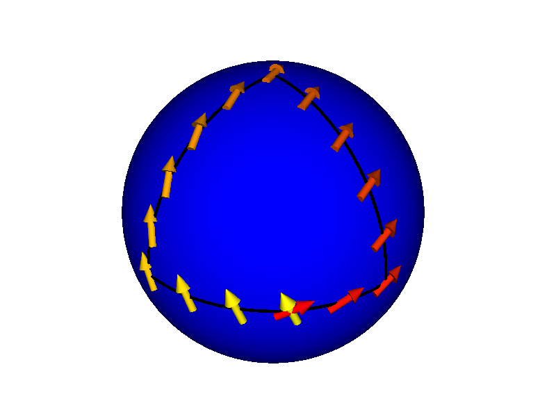
It must be emphasized that this precession has got nothing to do with the spin of the earth or the peculiarities of the latitude/longitude coordinate system. In figure 13 the sphere is completly abstract, with no spin, no latitude, no longitude, and no poles. As we shall see in section 10.4, the area of the loop is what matters, not the shape or orientation.
You can also see in figure 13 that the initial arrow does not need to be parallel or perpendicular to the path. Any initial orientation is allowed. The orientation of each successive arrow is dictated by the requirement that it be parallel to the previous arrow.
In all these diagrams, each new arrow is constructed to be parallel to the previous one, as parallel as it possibly could be. If you don’t see each successive arrow in this part of the diagram as being exactly parallel to the previous one, that’s because you live in three dimensions. Creatures who actually live in the curved space – the two-dimensional curved surface in this model system – cannot detect the third dimension.
This is related to the idea that the tape used in figure 1 is non-stretchy in two dimensions but is free to bend in the third dimension. We are modeling the physics as seen by creatures who live in the two-dimensional space. The third dimension – the embedding dimension – is not part of their world.
In particular, in the discussion associated with figure 9 we said that all the triangles keep their shape, whatever that shape might be. Now, if we impose the further requirement that the midpoint of line DB coincides with the midpoint of line AC, then we have similar triangles (indeed congruent triangles) and this guarantees that line BC is parallel to line AD. We use this to define what we mean by parallel transport. We use this construction – called Schild’s Ladder – to transport vector AD along the path AB and thereby prove, by construction, that it AD is parallel to BC.
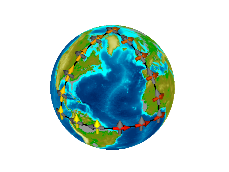
Here is another argument that leads to the same conclusion: The situation in figure 14 is very similar to the situation in figure 12. The main difference is that rather than having a single vector at each point, we have two vectors. This is one way of representing a bivector. (If the term “bivector” doesn’t mean anything to you, don’t worry about it.)
In particular, let’s look at the six bivectors on the leg of the triangle that goes through North America. Each of the gray vectors here points due west, along a “line” of constant latitude. Such “lines” are called parallels of latitude – as in the 49th parallel. They are indeed parallel, but they are not straight lines. That is to say, they are not geodesics (with one exception, namely the equator). So they are not “parallel lines” in the strict mathematical sense. In the embedding space they exist as circles in parallel planes. An short-enough segment of circle can be approximated by a straight line-segment, at at any given longitude these line-segments are parallel, as represented in figure 11 by the six gray arrows at 0∘ longitude, and also by the six gray arrows at 90∘ west longitude. Also if you treat them as existing in the D=2 surface they are parallel.
Once you are convinced that the gray arrows are parallel in these groups of six, the rest of the argument is easy. The yellowish arrows are perpendicular to the gray arrows. In two dimensions, this implies that the yellowish arrows must be parallel to one another. In two dimensions, there is no other possibility.
The amount of precession is proportional to the area enclosed by the loop, times the amount of curvature. In two dimensions we can write:
| (5) |
where dA is an element of area, and K denotes something we call the Gaussian curvature.
We can always define the average curvature (averaged over some area) as follows:
| (6) |
Then as an immediate corollary to equation 5 we obtain:
| (7) |
This gives us a convenient way of measuring the average curvature. Let’s see how it works for the spherical triangle shown in figure 12. The loop comprises one octant, i.e. one eighth of the area of the sphere. A sphere of radius R has curvature K = 1/R2 everywhere.
| (8) |
which is nicely consistent with equation 5 and equation 7.
Figure 15 is similar to Figure 12 except that the path encompasses a smaller area. You can see that there is correspondingly less precession.
Occasionally, we choose to imagine that our curved space is embedded in some higher-dimensional space. For example, the spherical surface shown in figure 12 is intrinsically a two-dimensional space. We only need two numers (e.g. latitude and longitude) to span the space. In this subsection, we imagine that it sits in a three-dimensional embedding space.
This allows us to write the Gaussian curvature in the form
| (9) |
where k1 is the principal curvature in one direction and k2 is the principal curvature in the other direction. For example, a sphere of radius R has k1 = k2 = 1/R everywhere, which is consistent with our previous assertion that K = 1/R2.
By way of constrast, a cylinder of radius R has zero Gaussian curvature, because k1 = 1/R but k2 = 0. The cylinder is curved in one direction but not the other. We can apply similar reasoning to a cone. We conclude that a cone has zero intrinsic curvature (except at the apex).
Each principal curvature is related to the corresponding radius of curvature:
| (10) |
It must be emphasized that r1, r2, k1, and k2 are extrinsic, and cannot be measured by the creatures who live in the two-dimensional space. In contrast, they can measure the intrinsic curvature, i.e. the Gaussian curvature K, by carrying out parallel-transport experiments and applying equation 7.
To demonstrate parallel transport using the same tabletop model shown in figure 1, proceed as follows:
From a strip of masking tape at least one inch wide, cut out a parallelogram. The exact shape doesn’t matter.
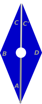
Draw the long diagonal on the parallelogram, as shown in figure 16. Use a pen with a moderate width, not too fine, for reasons that will become obvious in a moment. Label the corners {A, B, C, D}. Add another label, C′}, so that there are labels on both sides of the diagonal at corner C. For strain relief (aka crimp relief), make a keyhole-shaped cut, as shown in figure 16. That is, make a round hole in the middle, and then make a cut from the middle to corner C, running right down the middle of the line you marked. Try to cut the line in half. I found it easy to make the crimp-relief cuts by putting the tape on a firm board and using a scalpel (aka “hobbyist razor knife”). Using a scissors is possible but probably less convenient.
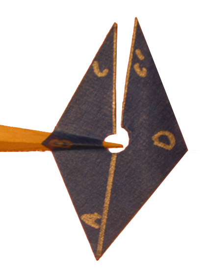
Lay the parallelogram on the model, so that the tip of a dart falls into the crimp-relief hole. I did it starting from point B and proceeding counterclockwise to point C′, then re-starting at point B and proceeding clockwise to point C. There are probably other satisfactory tactics. The result is shown in figure 17.
The parallel transport story goes like this: Start at point C. The initial vector that we wish to transport is the line that is drawn on the tape, the line that runs from the center to point C. We transport that via B, A, and D all the way to C′. The transported vector is now parallel to the line from the center to C′. Since the space between point C′ and point C is flat, you can easily use your imagination to transport the vector the rest of the way, all the way back to the starting point C. As you can see in figure 17, the vector has precessed by about 7 degrees.
If you look closely, you find that the direction of precession is the opposite of what we saw in figure 12. There if you go around the loop clockwise the precession is also clockwise, but here if you go around the loop clockwise the precession is counterclockwise. This is the hallmark of negative Gaussian curvature. A sheres has positive intrinsic curvature, while a saddle has negative intrinsic curvature.
Also: If you think about it for a while, and/or do some experiments with the model, you discover that for transport around any path that encompasses the tip of a dart, the amount of precession is the same, namely −7 degrees. The only way to describe this is to say that there is a Dirac delta-function of curvature, located at the tip of the dart.
If you don’t know what a delta-function is, don’t worry about it too much. In general, it’s just a fancy way of saying something is hugely concentrated, with a high density in one place and zero density elsewhere. Imagine a very tall, very narrow spike. In the present contect, when we talk about curvature, we are not talking about the curvature of the spike; the spike is not what’s curved. The space is curved, and the spike is telling us where the curvature is.
We can formalize this concentration of curvature as follows:
| (11) |
where θ is −7 degrees in this model, and the tip of the dart is located at the point (x0, y0). When we integrate this curvature in accordance with equation 5, we get the correct total precession. Note that a δ-function has units of inverse length, so the dimensions in equation 11 are correct.
Meanwhile for any path that encompasses the base of a dart, the precession is +7 degrees. In the model, there is no way to encompass the base of one dart without encompassing the base of its partner, so we see a total precession of +14. For any path that does not encompass the tip or base of any dart, there is no precession.
Tangential remark: If you carefully measure the angle in figure 17, you find that the angle is very close to −8 degrees, rather than the −7 that we were expecting based on the specifications of the darts. I don’t know whether this has to do with imperfections in the darts, or imperfections in the way I laid down the tape.
To repeat: To us, living in the embedding space, the darts may “look” like they have curvature all along their length, but really they don’t. They have zero intrinsic curvature except at the tips and bases. To say the same thing another way: the dart has one extrinsic curvature (k1) that is nonzero all along its length, but the other extrinsic curvature (k2) is zero, so the intrinsic Gaussian curvature is zero (except at the tip and the base).
As a consequence, the gravitational field that we are modeling in figure 12 is a piecewise-constant field. On the left side of the midline there is a field of constant strength pointing to the right, and on the right side of the midline there is a field of constant strength pointing to the left. This is similar to the field you would find in a three-plate parallel-plate capacitor, carrying a charge of −Q, +2Q, and −Q (respectively) on the plates.
In particular, in the main region of the diagram, between the tips and the bases of the darts, there is no geodesic deviation. As seen by creatures who live in the two-dimensional space, there is no spacetime curvature in this region. We who live in the embedding space see geodesics that seem to curve, but in this region they all curve together. A pair of geodesics that starts out parallel will remain parallel. That is to say, they do not deviate from each other, so there is no geodesic deviation.
The parallel geodesics remain parallel unless and until the pair straddles the tip or the base of a dart, whereupon there will be geodesic deviation. This is the fundamental mechanism of general relativity: Curvature causes geodesic deviation.
The analogy to real-world gravitation goes like this: Any region where the gravitational acceleration g is essentially uniform does not have any appreciable spacetime curvature. In particular, over the typical laboratory lengthscale, spacetime curvature is negligible. This is related to Einstein’s principle of equivalence, which says that a uniform gravitational field is indistinguishable from an acceleration of the reference frame. To say the same thing the other way, you can make a uniform gravitational field disappear by choosing a different reference frame. Therefore it is obvious that a uniform gravitational field has got nothing to do with spacetime curvature, because you can’t make curvature go away by choosing a different reference frame.
Many of the following fabrication ideas are due to Paul Fuoss.
Maple is an excellent material for making darts. (Any hard, fine-grained wood will do.) The grain should run down the long axis of the dart; this makes fabrication harder but makes the final result nicer. We found that Paul’s compound miter saw was the smart way to make them. We tried making them with a table saw but the compound miter saw was a much better choice.
Attach the hardwood piece (from which you are cutting the darts) to a much larger carrier piece, using wood screws, so you can hold it very securely without endangering your fingers. (Holding the piece securely is vastly more important for miter cuts than for regular cuts, where slight vertical motions are harmless.)
Each dart is a thin pyramid. The base of the pyramid is an equilateral triangle, 1/2 inch on a side. The pyramid is about 4 inch long in the other direction.
Set the saw so that the blade is inclined 30 degrees to the vertical. Then set it so that the arm is angled 3.6 degrees away from perpendicular to the fence. That gives a slope of 1 part in 16, i.e. 1/4 inch (half the base of the pyramid) per 4 inch.
Make the first cut. Cut just enough off one end of the stock so that the shape of the edge is determined by the cut. Then flip the stock over. If the stock was to the left of the blade to begin with, it will be to the right of the blade now. This may require unbolting the stock from the carrier and rebolting it (although you might avoid this step by using an extra-fancy carrier). Mark the starting point for the second cut. The base of the pyramid should be against the fence. Make the second cut. The first dart should fall free.
Jessica MacNaughton pointed out that you can make darts that are just as functional (but perhaps not as beautiful) out of clay. If you don’t have access to a compound miter saw, this may be your best option.
For an explanation of the concepts and notation used here, see reference 4.
We consider the motion of a free particle on the surface of the sphere. If all we cared about was spheres, there are lots of easy ways of describing the motion. We know the geodesics of a sphere are the great circles. However, let’s pretend we didn’t know that. The techniques used in this section work for spheres and non-spheres alike, even when the curvature varies from place to place in complicated ways. So this section is a warm-up exercise, intended to demonstrate the use of powerful tools by applying them to a relatively simple situation.
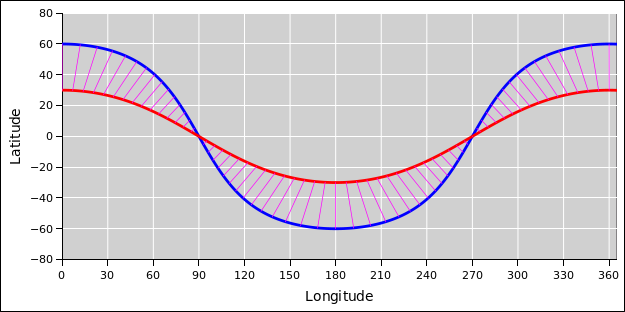
Figure 18 shows two trajectories on the sphere, one blue particle and one red particle. The trajectories look a bit odd, because this is a Mercator projection. Normally one should use something more sophisticaed than a Mercator projection, but in this section part of the goal is to show how to keep track of what’s going on, even in slightly non-ideal situations.
In the figure, each magenta tie-line connects the red particle at a given time with the blue particle at the same time. Both particles are moving at the same constant velocity. The spacing between tie-lines appears to change, but that’s just an artifact of the Mercator projection. Things near the pole get stretched sideways. A given east-west distance corresponds to less longitude near the equator and more longitude near the poles.
Let’s figure out how to calculate such things. Suppose a free particle starts out at a given position x with a given velocity v. At each time t, it is easy compute the new position a short time later:
| (12) |
Note that position component x1 is synonymous with θ, and component x2 is synonymous with φ.
In a curved space, it is nontrivial to calculate the new velocity. From the particle’s point of view, it feels like the velocity is unchanged, which stands to reason, since we are talking about a free particle. However, when we try to express this in components, the components of the velocity have changed.
To be specific, let’s assume ordinary spherical coordinates, namely longitude θ and latitude φ. For a free particle, θ· and φ· are constantly changing.† In contrast, maintaining constant θ· and φ· would correspond to following a rhumb line, not a great circle,† not a free-particle trajectory.†
Note † indicates statements that are true except on a set of measure zero. The exceptions correspond to following the equator or following a great circle through the poles, i.e. a line of longitude.
One way to make progress is to use the methods of classical mechanics, starting from the Lagrangian. As usual, the Lagrangian knows all and tells all. (A fancier solution to the same problem is discussed in section 12.3.)
For a free particle, the Lagrangian is just the kinetic energy. The mass doesn’t matter (assuming it is nonzero). It will drop out of the geodesic equation, so for simplicity we set it equal to 1. In polar coordinates the kinetic energy is:
| (13) |
assuming the particle speed is small compared to the speed of light. A slightly more general way of writing this is:
| (14) |
where g is the metric tensor, which will be discussed later; see equation 27.
In the usual way, the Lagrangian allows us to identify the momentum variable that is dynamically conjugate to each of our chosen position variables. For the free particle on a sphere, the momenta are:
| (15) |
Raising an index gives us an unsurprising result:
| (16) |
We can check these equations in various ways. For example we can check that the kinetic energy is:
| (17) |
Recall that we set m=1. Also in accordance with basic ideas of classical mechanics, the Hamiltonian is
| (18) |
So the Hamiltonian is equal to the Lagrangian, which comes as no surprise for a free particle.
For any Lagrangian, we can invoke the principle of least action to obtain the Euler-Lagrange equation, which is a nice way to express the equations of motion. The general form is:
| (19) |
It is instructive to check this by applying it to a well-understood system, such as a simple harmonic oscillator.
For the free particle on a sphere, we get:
| (20) |
and
| (21) |
That is all we need to calculate the curves in figure 18. See section 12.4 for some hints about numerical methods.
Here’s another solution to the same problem. This is a simplified version of the approach you see in books on general relativity. The fancy machinery used here is useful for a wide range of curvature-related and gravitation-related applications, not just geodesics, and not just spheres.
One simplification here is that the number of components in equation 23 is only 2×2×2 instead of 4×4×4 for general relativity. Furthermore, as we shall see, only three of the components are nonzero.
We expect that in general, the geodesic equation will tell us that the acceleration is bilinear in the velocity. The most general form for such an expression is:
| (22) |
where Γ embodies the information we have about the local curvature.
The components of Γ are called the Christoffel symbols. More specifically, the components Γijk are called the Christoffel symbols of the first kind, while the components Γijk (with a raised index) are called the Christoffel symbols of the second kind. We can display the components as follows:
| (23) |
In other words, the first component specifies which plane, the second component specifies which row, and the third component specifies which column. Imagine the two planes are stacked vertically to make a 2×2×2 cube, but we offset them for better visibility.
As we shall see, the components of Γ for a sphere are:
| (24) |
Plugging this into equation 22 we find:
| (25) |
which is consistent with equation 20 and equation 21. However at this point you should be wondering where we got equation 24. It turns out there is a general expression for the Christoffel symbols in terms of the metric, namely:
| (26) |
where the comma means to take the derivative. This expression can be derived using the notions of parallel transport as discussed in section 10. The basic idea is that the velocity vector is transported along the world-line in such a way that it stays parallel to itself and stays tangent to the world-line.
The metric for the 2-sphere (in spherical coordinates) is
| (27) |
The metric defines what we mean by dot product, which in turn defines what we mean by angle and distance. For example, equation 13 or equivalently equation 14 is just the dot product of the velocity with itself. An even simpler example uses plain old distance:
| (28) |
where ds is the element of arc length. If we combine the two previous equations it gives us another way to describe the metric of the sphere, namely:
| (29) |
You can verify that this metric is correct by thinking about the geometry of the sphere: how long is each line of constant longitude, and how long is each line of constant latitude.
If we differentiate this metric, the only nonzero component is:
| (30) |
It is then a matter of bookkeeping to figure out which three components of Γijk are nonzero, in accordance with equation 26. Then raise an index to obtain Γijk.
As a check, note that our Γijk in equation 24 is symmetric with respect to interchange of j and k. This is as it should be, as a consequence of equation 26 and the fact that gij itself is symmetric.
Let’s talk about what’s going on in terms of physics.
In figure 18, each particle is moving at constant speed along a great-circle route. Each particle, according to its own reckoning, is moving in a straight line. Each particle feels zero acceleration. Each particle is oblivious to the curvature. It is impossible in principle to measure the curvature using only one pointlike particle. Even the fact that each trajectory closes on itself does not demonstrate curvature. You could perfectly well have a flat space with periodic boundary conditions.
Things get much more interesting when we compare the two particles. They start out moving parallel to each other, but they don’t remain parallel. Each particle considers that the other is subject to a mysterious acceleration. In some sense it looks like gravitation. In particular, it looks like a tidal stress δg (not a simple acceleration g). The physical fact is that they accelerate relative to each other. This phenomenon is known as geodesic deviation.
For the spreadsheets used to do the calculations and prepare figure 18, see reference 7.
Hint #1: When doing the numerical integrations, first-order Euler is not good enough. Second-order Runge-Kutta (RK2) is good enough, if the stepsize is reasonably small (one degree or so) and the latitude is not too high (less than 70 degrees). One could imagine using fourth-order Runge-Kutta (RK4), but for the purposes of figure 18 it’s not worth the effort. Keep in mind that the coordinate system is singular at the poles, so there are limits to what you can hope to do.
Tangential remarks: If you switch to a better representation, you can get good results near the poles (and everywhere else). The physics doesn’t care what coordinate system – if any – you choose, and the physics is not singular. You can play catch near the north pole, and the ball will nicely obey all of Newton’s laws, just like anywhere else. Examples of better representations include:
- An airplane can maneuver in three dimensions. So we do not have a 2D spherical world embedded in an imaginary 3D space; we have a genuine 3D world. So it makes sense to represent the aircraft’s position as a 3D vector, namely (X, Y, Z), for all computational purposes. The velocity is also a 3D Cartesian vector. If desired, the (X, Y, Z) representation can be displayed as (latitude, longitude, altitude), provided the latitude is not too high. For polar travel, the internal (X, Y, Z) computations remain the same, but other display schemes are used; for example, there is a well-defined notion of “West Antarctica”.
- The attitude (i.e. orientation) of the aircraft is sometimes described in terms of three Euler angles – yaw, pitch, and roll – but those have terrible singularities at pitch=±90∘. The smart move is to switch to the bivector representation (aka quaternions) and then use Clifford algebra to compute changes in attitude. For the next level of detail on how this works, see reference 8 and reference 9. Every autopilot and every nontrivial flight simulator in the world does it this way.
There is no Cartesian representation of rotations in 3D or higher, because rotations around different axes do not commute. So you have to use bivectors (or matrices, or some other higher-dimensional representation).
- To calculate the great-circle route between point A and point B, it is super-easy to construct two 3D vectors (from the center of the earth to A and to B), then convert that into a bivector, and then use Clifford algebra to rotate things in the plane defined by that bivector. Again, see reference 8 and reference 9. To compute straight lines (i.e. geodesics) on the real earth, which is significantly ellipsoidal, takes a bit more work, but there are well-known formulas for that.
- In a sailboat or other conveyance restricted to the surface of a sphere, you can represent position using bivectors (aka quaternions). This works better than the (latitude, longitude) representation, especially at high latitudes. In particular, it accounts for the fact that “lines” of constant latitude are not straight lines. Another option is to embed the sphere in 3D space and use the (X, Y, Z) representation.
For present purposes we don’t need to know any of that. We can get by with polar coordinates if we’re careful.
Hint #2: As usual when applying Runge-Kutta to a system of differential equations, a useful trick is to reduce it to a single differential equation with more components. In this case the crucial variable is a vector with four components:
| (31) |
where we define
| (32) |
Loosely speaking, X is a point in phase space. Non-loosely speaking, remember that the coordinates in phase space are (position, momentum) not (position, velocity), and one of the momenta has a factor of cos2 in accordance with equation 15.
When we differentiate equation 31 and plug in equation 32 and equation 25 we find:
| (33) |
The first two rows in equation 33 may appear trivial, but they are an important part of the game. Overall equation 33 gives us a nice simple expression for X· in terms of X, which we can integrate using RK.
Beware that integrating equation 33 is probably not optimal. It would probably be smarter to build a symplectic integrator, but that’s more work than I feel like doing at the moment. It’s work, because the Lagrangian is not easily separable. This stands in contrast to the Lagrangian for simple mechanics problems, where the force depends only on position, not on velocity. Even though it’s not easily separable, the geodesic equation is still undoubtedly conservative and reversible, so we “should” be able to build a symplectic integrator somehow. See reference 10.
Hint #3: As always, some good advice is:
Following this advice may slightly increase the workload in the short run, but it greatly reduces the workload in the long run, especially when dealing with complex problems. For details on this, see reference 11.
In that spirit, the spreadsheet in reference 7 calculates the speed of the particle at each step. If this is appreciably non-constant, it indicates a defect in the calculation. You can generally tell by looking at the plot that there’s something wrong, but the speed provides a way of quantifying the problem.
Here’s another instructive exercise, even simpler than the previous one: Calculate the geodesics in a plane, i.e. a flat two-dimensional plane. To make it interesting, use polar coordinates.
In this situation there is no tidal stress and no geodesic deviation. However, the geodesic equation is nontrivial, because the coordinate basis {dr, dθ} means different things in different places, and the equation of motion must take this into account.
One advantage here is that it is super-easy to graph the results, and there’s no doubt about how to interpret the graph.
If you want to understand gravitational waves, the first step is to have a clear understanding of what gravitation is. See reference 12.
In particular, the distinction between the framative acceleration g and the massogenic tidal stress δg is often underappreciated. Note that g is completely frame-dependent, whereas δg is completely frame-independent. If you’re looking for gravitational waves, you need to look for tidal stress.
By way of analogy, it is not possible to explain electromagnetic radiation in any direct way starting from the electrostatic interaction. There are lots of introductory textbooks that claim to do this, but it’s nonsense. In the Liénard-Wiechert potentials, the term that is needed to explain radiation does not appear in Coulomb’s law. See reference 13.
By the same token, it is not possible to explain a gravitational wave in terms of the Newton’s law of gravitation. If you try, you’ll get the wrong polarization, the wrong dependence on frequency, the wrong dependence on distance, et cetera. You might be able to make something happen in the near-field region, but it’s not really a wave. It doesn’t propagate properly. In the far field, it does not exist.
Here’s the concept map:
| Electrostatics | | Electrodynamics | | Electromagnetic Waves |
| (Coulomb) | | (Maxwell) | | (Larmor) |
| | | |||
| Static Gravitation | | Dynamic Gravitation | | Gravitational Waves |
| (Newton) | | (Einstein) | | (section 13.3) |
The point is, the interesting analogy moves vertically from electromagnetic waves to gravitational waves (not starting from static Newtonian gravity). The Larmor formula is discussed in section 13.2 and the corresponding idea is applied to gravitational waves in section 13.3.
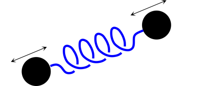
The canonical Gedankenexperiment for transmitting gravitational waves is shown in figure 19. It is a mechanical oscillator, with two masses connected by a spring. The masses move 180 degrees out of phase, so that the center of mass remains stationary.
The distribution of mass in the transmitter has a time-dependent quadrupole moment. (This is analogous to an electromagnetic transmitter with a time-dependent dipole moment.)
|
| |
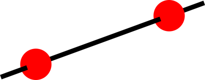
| Figure 19: Gravitational Wave Transmitter | Figure 20: Detector: Beads Sliding on a Stick | |
The canonical receiver is shown in figure 20. It has two beads that are free to slide along a stick. The beads are what’s important; the stick is just there to give us a robust operational definition of distance, so we don’t go crazy.
By way of contrast, if we just had a loose collection of dust particles, it would be very unwise to lay out an X axis by marking some of the particles. When the wave came along, each and every particle would move as a free particle, oblivious to the wave. None of the particles would move relative to the bogus local X axis. The stick in figure 20 is not an abstract axis but rather a sturdy mechanical stick. When the wave comes along, it sets up some tidal stress in the stick, but the atoms in the stick do not respond as free particles. To a very good approximation they do not move at all relative to one another. The atoms resist the stress and maintain their size, as set by the laws of atomic physics.
When the wave comes along, the beads accelerate relative to one another. If we add a tiny amount of friction, the stick heats up, leaving indisputable evidence of the effect of the wave.
Tidal stress on the stick produces an exceedingly small strain; tidal stress on beads, dust, and other free particles produces a much larger strain.
For details on all this, see reference 14 and reference 15.
It is an amusing exercise to derive the Larmor formula for the total radiated power using little more than scaling arguments. You can then obtain the gravitational wave formula in the same way.
Suppose we have an oscillating electric dipole. The radiated power cannot depend on the dipole moment itself; otherwise a static dipole would radiate, which would not make sense physically. Similarly the power cannot depend on the time derivative of the dipole moment, because two charged particles moving past each other in uniform straight-line motion cannot possibly radiate. Neither one radiates by itself, so (by superposition) they cannot radiate together ... yet this configuration has a time-varying dipole moment. So the lowest term that makes sense is the second time derivative of the dipole moment.
Step 2: The radiated power must depend on the square of that, for any number of reasons including symmetry with respect to flipping the definition of positive versus negative charge. Also we know that the fields are proportional to the dipole moment, and the energy goes like the square of the field.
Step 3: We need a factor of 1/є0 out front, to get something with dimensions of energy (as opposed to field strength). Then we need a factor of 1/c3 to make the dimensions come out right.
Step 4: If you want the received power per unit area at some distance r from the source, divide by 1/r2. Also at this point you need to worry about polarization and other directional effects, but let’s not worry about that.
Conceptually, that’s all there is to it. There are some factors of π running around, but let’s not worry about that. We have a perfectly reasonable feel for what’s going on.
We can replay the ideas from section 13.2 and apply them do gravitational waves.
You can’t have a mass dipole, so the lowest-order thing we need to worry about is the quadrupole moment. (If you want to get fancy, it’s the reduced quadrupole moment, but let’s not worry about that.)
It can’t be the quadrupole moment, or the first time derivative, or even the second time derivative thereof, because otherwise two masses moving past each other in uniform straight-line motion would radiate, and we know that’s not going to happen. So the object of interest is the third time derivative of the reduced quadrupole moment.
Step 2: The radiated gravitational-wave power must depend on the square of that, for any number of reasons including time-reversal symmetry. Also we should be very unsurprised to find that the energy goes like the square of the field strength.
Step 3: We need a factor of capital G out front, to get something with units of energy (as opposed to field strength). Then we need a factor of 1/c5 to make the dimensions come out right.
Step 4: If you want the received power per unit area at some distance r from the source, divide by 1/r2. Also at this point you need to worry about polarization and other directional effects, but let’s not worry about that.
Conceptually, that’s all there is to it. There are some factors of 2 running around, but let’s not worry about that. We have a perfectly reasonable feel for what’s going on.
Note that G is small, 1/c5 is small, and ω6 is small for typical events involving massive objects. So we are not surprised to hear that the gravitational waves are weak.
"The description of right lines and circles, upon which geometry is founded, belongs to mechanics. Geometry does not teach us to draw these lines, but requires them to be drawn."
– Sir Isaac Newton
(preface to the Principia)