Feynman defined equilibrium to be “when all the fast things have happened but the slow things have not” (reference 28). That statement pokes fun at the arbitrariness of the split between “fast” and “slow” – but at the same time it is 100% correct and insightful. There is an element of arbitrariness in our notion of equilibrium. Note the following contrast:
| Over an ultra-long timescale, a diamond will turn into graphite. | Over an ultra-short timescale, you can have non-equilibrium distributions of phonons rattling around inside a diamond crystal, such that it doesn’t make sense to talk about the temperature thereof. |
| Usually thermodynamics deals with the intermediate timescale, long after the phonons have become thermalized but long before the diamond turns into graphite. During this intermediate timescale it makes sense to talk about the temperature, as well as other thermodynamic properties such as volume, density, entropy, et cetera. |
One should neither assume that equilibrium exists, nor that it doesn’t.
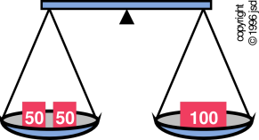
The word equilibrium is quite ancient. The word has the same stem as the name of the constellation “Libra” — the scale. The type of scale in question is the two-pan balance shown in figure 10.1, which has been in use for at least 7000 years.
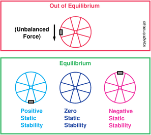
The notion of equilibrium originated in mechanics, long before thermodynamics came along. The compound word “equilibrium” translates literally as “equal balance” and means just that: everything in balance. In the context of mechanics, it means there are no unbalanced forces, as illustrated in the top half of figure 10.2.
Our definition of equilibrium applies to infinitely large systems, to microscopic systems, and to everything in between. This is important because in finite systems, there will be fluctuations even at equilibrium. See section 10.8 for a discussion of fluctuations and other finite-size effects.
The idea of equilibrium is one of the foundation-stones of thermodynamics ... but any worthwhile theory of thermodynamics must also be able to deal with non-equilibrium situations.
Consider for example the familiar Carnot heat engine: It depends on having two heat reservoirs at two different temperatures. There is a well-known and easily-proved theorem (section 14.4) that says at equilibrium, everything must be at the same temperature. Heat bath #1 may be internally in equilibrium with itself at temperature T1, and heat bath may be internally in equilibrium with itself at temperature T2, but the two baths cannot be in equilibrium with each other.
So we must modify Feynman’s idea. We need to identify a timescale of interest such that all the fast things have happened and the slow things have not. This timescale must be long enough so that certain things we want to be in equilibrium have come into equilibrium, yet short enough so that things we want to be in non-equilibrium remain in non-equilibrium.
Here’s another everyday example where non-equilibrium is important: sound. As you know, in a sound wave there will be some points where the air is compressed an other points, a half-wavelength away, where the air is expanded. For ordinary audible sound, this expansion occurs isentropically not isothermally. It you analyze the physics of sound using the isothermal compressibility instead of the isentropic compressibility, you will get the wrong answer. Among other things, your prediction for the speed of sound will be incorrect. This is an easy mistake to make; Isaac Newton made this mistake the first time he analyzed the physics of sound.
Again we invoke the theorem that says in equilibrium, the whole system must be at the same temperature. Since the sound wave is not isothermal, and cannot even be satisfactorily approximated as isothermal, we conclude that any worthwhile theory of thermodynamics must include non-equilibrium thermodynamics.
For a propagating wave, the time (i.e. period) scales like the distance (i.e. wavelength). In contrast, for diffusion and thermal conductivity, the time scales like distance squared. That means that for ultrasound, at high frequencies, a major contribution to the attenuation of the sound wave is thermal conduction between the high-temperature regions (wave crests) and the low-temperature regions (wave troughs). If you go even farther down this road, toward high thermal conductivity and short wavelength, you can get into a regime where sound is well approximated as isothermal. Both the isothermal limit and the isentropic limit have relatively low attenuation; the intermediate case has relatively high attenuation.
Questions of efficiency are central to thermodynamics, and have been since Day One (reference 29).
For example in figure 1.3, if we try to extract energy from the battery very quickly, using a very low impedance motor, there will be a huge amount of power dissipated inside the battery, due to the voltage drop across the internal series resistor R1. On the other hand, if we try to extract energy from the battery very slowly, most of the energy will be dissipated inside the battery via the shunt resistor R2 before we have a chance to extract it. So efficiency requires a timescale that is not too fast and not too slow.
Another example is the familiar internal combustion engine. It has a certain tach at which it works most efficiently. The engine is always nonideal because some of the heat of combustion leaks across the boundary into the cylinder block. Any energy that goes into heating up the cylinder block is unavailable for doing P DV work. This nonideality becomes more serious when the engine is turning over slowly. On the other edge of the same sword, when the engine is turning over all quickly, there are all sorts of losses due to friction in the gas, friction between the mechanical parts, et cetera. These losses increase faster than linearly as the tach goes up.
If you have gas in a cylinder with a piston and compress it slowly, you can (probably) treat the process as reversible. On the other hand, if you move the piston suddenly, it will stir the gas. This can be understood macroscopically in terms of sound radiated into the gas, followed by frictional dissipation of the sound wave (section 11.5.1). It can also be understood microscopically in terms of time-dependent perturbation theory; a sudden movement of the piston causes microstate transitions that would otherwise not have occurred (section 11.5.2).
Another of the great achievements of thermodynamics is the ability to understand what processes occur spontaneously (and therefore irreversibly) and what processes are reversible (and therefore non-spontaneous). The topic of spontaneity, reversibility, stability, and thermodynamic equilibrium is discussed in depth in chapter 14.
Any theory of thermodynamics that considers only reversible processes – or which formulates its basic laws and concepts in terms of reversible processes – is severely crippled.
If you want to derive the rules that govern spontaneity and irreversibility, as is done in chapter 14, you need to consider perturbations away from equilibrium. If you assume that the perturbed states are in equilibrium, the derivation is guaranteed to give the wrong answer.
In any reversible process, entropy is a conserved quantity. In the real world, entropy is not a conserved quantity.
If you start with a reversible-only equilibrium-only (ROEO) theory of thermodynamics and try to extend it to cover real-world situations, it causes serious conceptual difficulties. For example, consider an irreversible process that creates entropy from scratch in the interior of a thermally-isolated region. Then imagine trying to model it using ROEO ideas. You could try to replace the created entropy by entropy the flowed in from some fake entropy reservoir, but that would just muddy up the already-muddy definition of heat. Does the entropy from the fake entropy reservoir count as “heat”? The question is unanswerable. The “yes” answer is unphysical since it violates the requirement that the system is thermally isolated. The “no” answer violates the basic conservation laws.
Additional examples of irreversible processes that deserve our attention are discussed in sections 10.3, 11.5.1, 11.5.3, 11.5.5, and 11.6.
Any theory of reversible-only equilibrium-only thermodynamics is dead on arrival.
The basic ideas of stability and equilibrium are illustrated in figure 10.2. (A more quantitative discussion of stability, equilibrium, spontaneity, reversibility, etc. can be found in chapter 14.)
We can understand stability as follows: Suppose we have two copies (two instances) of the same system. Suppose the initial condition of instance A is slightly different from the initial condition of instance B. If the subsequent behavior of the two copies remains closely similar, we say the system is stable.
More specifically, we define stability as follows: If the difference in the behavior is proportionate to the difference in initial conditions, we say the system is stable. Otherwise it is unstable. This notion of stability was formalized by Lyapunov in the 1880s, although it was understood in less-formal ways long before then.
For a mechanical system, such as in figure 10.2, we can look into the workings of how equilibrium is achieved. In particular,
Note that the equilibrium position in system B is shifted relative to the equilibrium position in system A. Stability does not require the system to return to its original position. It only requires that the response be proportionate to the disturbance.
If rather than applying a force, we simply move this system to a new position, it will be at equilibrium at the new position. There will be infinitely many equilibrium positions.
For a non-mechanical system, such as a chemical reaction system, corresponding ideas apply, although you have to work harder to define the notions that correspond to displacement, applied force, restoring force, et cetera.
A system with positive static stability will be stable in the overall sense, unless there is a lot of negative damping or something peculiar like that.
Note that a system can be stable with respect to one kind of disturbance but unstable with respect to another. As a simple example, consider the perfectly balanced wheel, with no damping.
To determine stability, normally you need to consider all the dynamical variables. In the previous example, the long-term velocity difference is bounded, but that doesn’t mean the system is stable, because the long-term position is unbounded.
Properly speaking, a system with zero stability can be called “neutrally unstable”. More loosely speaking, sometimes a system with zero stability is called “neutrally stable”, although that is a misnomer. A so-called “neutrally stable” system is not stable, just as “zero money” is not the same as “money”.
Tangential remark: In chemistry class you may have heard of “Le Châtelier’s principle”. Ever since Le Châtelier’s day there have been two versions of the “principle”, neither of which can be taken seriously, for reasons discussed in section 14.9.
To reiterate: Stability means that two systems that start out with similar initial conditions will follow similar trajectories. Sometimes to avoid confusion, we call this the “overall” stability or the “plain old” stability ... but mostly we just call it the stability.
Meanwhile, static stability arises from a force that depends on position of the system. In contrast, damping refers to a force that depends on the velocity.
The term “dynamic stability” is confusing. Sometimes it refers to damping, and sometimes it refers to the plain old stability, i.e. the overall stability. The ambiguity is semi-understandable and usually harmless, because the only way a system can have positive static stability and negative overall stability is by having negative damping.
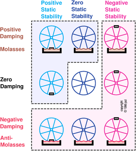
Static stability can be positive, zero, or negative; damping can also be positive, zero, or negative. A dynamical system can display any combination of these two properties — nine possibilities in all, as shown in figure 10.3. In the top row, the bicycle wheel is dipped in molasses, which provides damping. In the middle row, there is no damping. In the bottom row, you can imagine there is some hypothetical “anti-molasses” that provides negative damping.
The five possibilities in the bottom row and the rightmost column have negative overall stability, as indicated by the pale-red shaded region. The three possibilities nearest the upper-left corner have positive overall stability, as indicated by the pale-blue shaded region. The middle possibility (no static stability and no damping) is stable with respect to some disturbances (such as a change in initial position) but unstable with respect to others (such as a change in initial velocity).
By the way: Damping should be called “damping” not “dampening” — if you start talking about a “dampener” people will think you want to moisten the system.
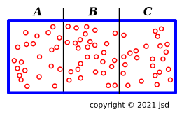
In figure 10.4, we initially have three separate systems — A, B, and C — separated by thin partitions. They are meant to be copies of each other, all in the same thermodynamic state. Then we pull out the partitions. We are left with a single system — ABC — with three times the energy, three times the entropy, three times the volume, and three times the number of particles.
Suppose we have a system where the energy can be expressed as a function of certain other extensive variables:
| (10.1) |
Note: If there are multiple chemical components, then N is a vector, with components Nν.
In any case, it is convenient and elegant to lump the variables on the RHS into a vector X with components Xi for all i. (This X does not contain all possible extensive variables; just some selected set of them, big enough to span the thermodynamic state space. In particular, E is extensive, but not included in X.)
We introduce the general mathematical notion of homogeneous function as follows. Let α be a scalar. If we have a function with the property:
| (10.2) |
then we say the function E is homogeneous of degree k.
Applying this to thermo, we say the energy is a homogeneous function of the selected extensive variables, of degree k=1.
It is amusing to differentiate equation 10.2 with respect to α, and then set α equal to 1.
| (10.3) |
There are conventional names for the partial derivatives on the LHS: temperature, −pressure, and chemical potential, as discussed in section 7.4. Note that these derivaties are intensive (not extensive) quantities. Using these names, we get:
| (10.4) |
which is called Euler’s thermodynamic equation. It is a consequence of the fact that the extensive variables are extensive. It imposes a constraint, which means that not all of the variables are independent.
If there are multiple chemical components, this generalizes to:
| (10.5) |
If we take the exterior derivative of equation 10.4 we obtain:
| (10.6) |
The red terms on the LHS are just the expanded form of the gradient of E, expanded according to the chain rule, as discussed in connection with equation 7.5 in section 7.4. Subtracting this from both sides gives us:
| (10.7) |
which is called the Gibbs-Duhem equation. It is a vector equation (in contrast to equation 10.4, which is a scalar equation). It is another way of expressing the contraint that comes from the fact that the extensive variables are extensive.
This has several theoretical ramifications as well as practical applications.
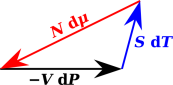
For starters: It may be tempting to visualize the system in terms of a thermodynamic state space where dT, dP, and dµ are orthogonal, or at least linearly independent. However, this is impossible. In fact dµ must lie within the two-dimensional state space spanned by dT and dP. We know this because a certain weighted sum has to add up to zero, as shown in figure 10.5.
Technical note: For most purposes it is better to think of the ectors dT, dP, and dµ as one-forms (row vectors) rather than pointy vectors (column vectors), for reasons discussed in reference 4. However, equation 10.7 is a simple linear-algebra proposition, and it can be visualized in terms of pointy vectors. There’s no harm in temporarily using the pointy-vector representation, and it makes the vector-addition rule easier to visualize.
As we shall discuss, finite size effects can be categorized as follows (although there is considerable overlap among the categories):
We shall see that:
Let’s start with an example: The usual elementary analysis of sound in air considers only adiabatic changes in pressure and density. Such an analysis leads to a wave equation that is non-dissipative. In reality, we know that there is some dissipation. Physically the dissipation is related to transport of energy from place to place by thermal conduction. The amount of transport depends on wavelength, and is negligible in the hydrodynamic limit, which in this case means the limit of very long wavelengths.
We can come to the same conclusion by looking at things another way. The usual elementary analysis treats the air in the continuum limit, imagining that the gas consists of an infinite number density of particles each having infinitesimal size and infinitesimal mean free path. That’s tantamount to having no particles at all; the air is approximated as a continuous fluid. In such a fluid, sound would travel without dissipation.
So we have a macroscopic view of the situation (in terms of nonzero conductivity) and a microscopic view of the situation (in terms of quantized atoms with a nonzero mean free path). These two views of the situation are equivalent, because thermal conductivity is proportional to mean free path (for any given heat capacity and given temperature).
In any case, we can quantify the situation by considering the ratio of the wavelength Λ to the mean free path λ. Indeed we can think in terms of a Taylor series in powers of λ/Λ.
Let us now discuss fluctuations.
As an example, in a system at equilibrium, the pressure as measured by a very large piston will be essentially constant. Meanwhile, the pressure as measured by a very small piston will fluctuate. These pressure fluctuations are closely related to the celebrated Brownian motion.
Fluctuations are the rule, whenever you look closely enough and/or look at a small enough subsystem. There will be temperature fluctuations, density fluctuations, entropy fluctuations, et cetera.
We remark in passing that the dissipation of sound waves is intimately connected to the fluctuations in pressure. They are connected by the fluctuation / dissipation theorem, which is a corollary of the second law of thermodynamics.
There is magnificent discussion of fluctuations in Feynman volume I chapter 46 (“Ratchet and Pawl”). See reference 8.
As another example, consider shot noise. That is: in a small-sized electronic circuit, there will be fluctuations in the current, because the current is not carried by a continuous fluid but rather by electrons which have a quantized charge.
Let us now discuss boundary terms.
If you change the volume of a sample of compressible liquid, there is a well-known P dV contribution to the energy, where P is the pressure and V is the volume. There is also a τ dA contribution, where τ is the surface tension and A is the area.
A simple scaling argument proves that for very large systems, the P dV term dominates, whereas for very small systems the τ dA term dominates. For moderately large systems, we can start with the P dV term and then consider the τ dA term as a smallish correction term.
In more detail:
Just because a reaction proceeds faster at high temperature does not mean it is exothermic. As a familiar example, the combustion of coal is famously exothermic, yet it proceeds much faster at elevated temperature.
Temperature is not the same as catalysis, insofar as sometimes it changes the equilibrium point. However, you can’t infer the equilibrium point or the energy balance just by casual obseration of the temperature.