In science, questions are not decided by taking votes, or by seeing who argues the loudest or the longest. Scientific questions are decided by a careful combination of experiments and reasoning. So here are some epochal experiments that form the starting point for the reasoning presented here, and illustrate why certain other approaches are unsatisfactory.
Make a bunch of thermometers. Calibrate them, to make sure they agree with one another. Use thermometers to measure each of the objects mentioned below.
In contrast, energy and entropy are extensive quantities, to an excellent approximation, for macroscopic systems. Each sub-parcel has half as much energy and half as much entropy as the original large parcel.
The terms intensive and extensive are a shorthand way of expressing simple scaling properties. Any extensive property scales like the first power of any other extensive property, so if you know any extensive property you can recognize all the others by their scaling behavior. Meanwhile, an intensive property scales like the zeroth power of any extensive property.
(This can be seen to be related to the previous point, if we consider two bodies that are simply parts of a larger body.)
Here is a collection of observed phenomena that tend to support equation 9.1.
| rate = A e−Ea / kT (11.1) |
where Ea is called the activation energy and the prefactor A is called the attempt frequency . The idea here is that the reaction pathway has a potential barrier of height Ea and the rate depends on thermal activation over the barrier. In the independent-particle approximation, we expect that thermal agitation will randomly give an exponentially small fraction of the particles an energy greater than Ea in accordance with equation 9.1.
Of course there are many examples where equation 11.1 would not be expected to apply. For instance, the flow of gas through a pipe (under the influence of specified upstream and downstream pressures) is not a thermally activated process, and does not exhibit an exponential dependence on inverse temperature.
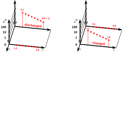
Consider an ordinary electrical battery. This is an example of a system where most of the modes are characterized by well-defined temperature, but there are also a few exceptional modes. Often such systems have an energy that is higher than you might have guessed based on the temperature and entropy, which makes them useful repositories of “available” energy.
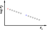
Figure 11.1 shows the probability of the various microstates of the battery, when it is discharged (on the left) or charged (on the right). Rather that labeling the states by the subscript i as we have done in the past, we label them using a pair of subscripts i,j, where i takes on the values 0 and 1 meaning discharged and charged respectively, and j runs over the thermal phonon modes that we normally think of as embodying the heat capacity of an object.
Keep in mind that probabilities such as Pi,j are defined with respect to some ensemble. For the discharged battery at temperature T, all members of the ensemble are in contact with a heat bath at temperature T. That means the thermal phonon modes can exchange energy with the heat bath, and different members of the ensemble will have different amounts of energy, leading to the probabilistic distribution of energies shown on the left side of figure 11.1. The members of the ensemble are not able to exchange electrical charge with the heat bath (or with anything else), so that the eight microstates corresponding to the charged macrostate have zero probability. It doesn’t matter what energy they would have, because they are not accessible. They are not in equilibrium with the other states.
Meanwhile, on the right side of the figure, the battery is in the charged state. The eight microstates corresponding to the discharged macrostate have zero probability, while the eight microstates corresponding to the charged macrostate have a probability distribution of the expected Boltzmann form.
Comparing the left side with the right side of figure 11.1, we see that the two batteries have the same temperature. That is, the slope of log(Pi,j) versus Ei,j – for the modes that are actually able to contribute to the heat capacity – is the same for the two batteries.
You may be wondering how we can reconcile the following four facts: (a) The two batteries have the same temperature T, (b) the accessible states of the two batteries have different energies, indeed every accessible state of the charged battery has a higher energy than any accessible state of the discharged battery, (c) corresponding accessible states of the two batteries have the same probabilities, and (d) both batteries obey the Boltzmann law, Pi,j proportional to exp(−Ei,j/kT). The answer is that there is a bit of a swindle regarding the meaning of “proportional”. The discharged battery has one proportionality constant, while the charged battery has another. For details on this, see section 24.1.
Here is a list of systems that display this sort of separation between thermal modes and nonthermal modes:
(Section 11.4 takes another look at metastable systems.)
There are good reasons why we might want to apply thermodynamics to systems such as these. For instance, the Clausius-Clapeyron equation can tell us interesting things about a voltaic cell.
Also, just analyzing such a system as a Gedankenexperiment helps us understand a thing or two about what we ought to mean by “equilibrium”, “temperature”, “heat”, and “work”.
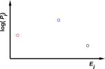
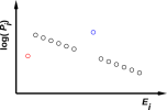
In equilibrium, the “accessible” states are supposed to be occupied in accordance with the Boltzmann distribution law (equation 9.1).
An example is depicted in figure 11.1, which is a scatter plot of Pi,j versus Ei,j.
As mentioned in section 10.1, Feynman defined equilibrium to be “when all the fast things have happened but the slow things have not” (reference 28). The examples listed at the beginning of this section all share the property of having two timescales and therefore two notions of equilibrium. If you “charge up” such a system you create a Boltzmann distribution with exceptions. There are not just a few exceptions as in figure 11.3, but huge classes of exceptions, i.e. huge classes of microstates that are (in the short run, at least) inaccessible. If you revisit the system on longer and longer timescales, eventually the energy may become dissipated into the previously-inaccessible states. For example, the battery may self-discharge via some parasitic internal conduction path.
|
| |
| Figure 11.2: An Equilibrium Distribution | Figure 11.3: An Equilibrium Distribution with Exceptions | |
The idea of temperature is valid even on the shorter timescale. In practice, I can measure the temperature of a battery or a flywheel without waiting for it to run down. I can measure the temperature of a bottle of H2O2 without waiting for it to decompose.
This proves that in some cases of interest, we cannot write the system energy E as a function of the macroscopic thermodynamic variables V and S. Remember, V determines the spacing between energy levels (which is the same in both figures) and S tells us something about the occupation of those levels, but alas S does not tell us everything we need to know. An elementary example of this can be seen by comparing figure 9.1 with figure 11.3, where we have the same V, the same S, and different E. So we must not assume E = E(V,S). A more spectacular example of this can be seen by comparing the two halves of figure 11.1.
Occasionally somebody tries to argue that the laws of thermodynamics do not apply to figure 11.3 or figure 11.1, on the grounds that thermodynamics requires strict adherence to the Boltzmann exponential law. This is a bogus argument for several reasons. First of all, strict adherence to the Boltzmann exponential law would imply that everything in sight was at the same temperature. That means we can’t have a heat engine, which depends on having two heat reservoirs at different temperatures. A theory of pseudo-thermodynamics that cannot handle exceptions to the Boltzmann exponential law is useless.
So we must allow some exceptions to the Boltzmann exponential law … maybe not every imaginable exception, but some exceptions. A good criterion for deciding what sort of exceptions to allow is to ask whether it is operationally possible to measure the temperature. For example, in the case of a storage battery, it is operationally straightforward to design a thermometer that is electrically insulated from the exceptional mode, but thermally well connected to the thermal modes.
Perhaps the most important point is that equation 1.1 and equation 2.1 apply directly, without modification, to the situations listed at the beginning of this section. So from this point of view, these situations are not “exceptional” at all.
The examples listed at the beginning of this section raise some other basic questions. Suppose I stir a large tub of water. Have I done work on it (w) or have I heated it (q)? If the question is answerable at all, the answer must depend on timescales and other details. A big vortex can be considered a single mode with a huge amount of energy, i.e. a huge exception to the Boltzmann distribution. But if you wait long enough the vortex dies out and you’re left with just an equilibrium distribution. Whether you consider this sort of dissipation to be q and/or heat is yet another question. (See section 7.10 and especially section 17.1 for a discussion of what is meant by “heat”.)
In cases where the system’s internal “spin-down” time is short to all other timescales of interest, we get plain old dissipative systems. Additional examples include:
An interesting example is:
In this case, it’s not clear how to measure the temperature or even define the temperature of the spin system. Remember that in equilibrium, states are supposed to be occupied with probability proportional to the Boltzmann factor, Pi ∝ exp(−Êi/kT). However, the middle microstate is more highly occupied than the microstates on either side, as depicted in figure 11.4. This situation is clearly not describable by any exponential, since exponentials are monotone.
We cannot use the ideas discussed in section 11.3 to assign a temperature to such a system, because it has so few states that we can’t figure out which ones are the thermal “background” and which ones are the “exceptions”.
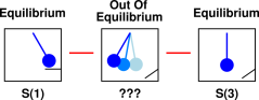
Such a system does have an entropy – even though it doesn’t have a temperature, even though it is metastable, and even though it is grossly out of equilibrium. It is absolutely crucial that the system system have a well-defined entropy, for reasons suggested by figure 11.5. That is, suppose the system starts out in equilibrium, with a well-defined entropy S(1). It then passes through in intermediate state that is out of equilibrium, and ends up in an equilibrium state with entropy S(3). The law of paraconservation of entropy is meaningless unless we can somehow relate S(3) to S(1). The only reasonable way that can happen is if the intermediate state has a well-defined entropy. The intermediate state typically does not have a temperature, but it does have a well-defined entropy.
Consider the apparatus shown in figure 11.6. You can consider it a two-sided piston.
Equivalently you can consider it a loudspeaker in an unusual full enclosure. (Loudspeakers are normally only half-enclosed.) It is roughly like two unported speaker enclosures face to face, completely enclosing the speaker driver that sits near the top center, shown in red. The interior of the apparatus is divided into two regions, 1 and 2, with time-averaged properties (E1, S1, T1, P1, V1) and (E2, S2, T2, P2, V2) et cetera. When the driver (aka piston) moves to the right, it increase volume V1 and decreases volume V2. The box as a whole is thermally isolated / insulated / whatever. That is to say, no entropy crosses the boundary. No energy crosses the boundary except for the electricity feeding the speaker.
You could build a simplified rectangular version of this apparatus for a few dollars. It is considerably easier to build and operate than Rumford’s cannon-boring apparatus (section 11.5.3).
We will be primarily interested in a burst of oscillatory motion. That is, the piston is initially at rest, then oscillates for a while, and then returns to rest at the original position.
When the piston moves, it does F·dx work against the gas. There are two contributions. Firstly, the piston does work against the gas in each compartment. If P1 = P2 this contribution vanishes to first order in dV. Secondly, the piston does work against the pressure in the sound field.
The work done against the average pressure averages to zero over the course of one cycle of the oscillatory motion ... but the work against the radiation field does not average to zero. The dV is oscillatory but the field pressure is oscillatory too, and the product is positive on average.
The acoustic energy radiated into the gas is in the short term not in thermal equilibrium with the gas. In the longer term, the sound waves are damped i.e. dissipated by internal friction and also by thermal conductivity, at a rate that depends on the frequency and wavelength.
What we put in is F·dx (call it “work” if you wish) and what we get out in the long run is an increase in the energy and entropy of the gas (call it “heat” if you wish).
It must be emphasized that whenever there is appreciable energy in the sound field, it is not possible to write E1 as a function of V1 and S1 alone, or indeed to write E1 as a function of any two variables whatsoever. In general, the sound creates a pressure P(r) that varies from place to place as a function of the position-vector r. That’s why we call it a sound field; it’s a scalar field, not a simple scalar.
As a consequence, when there is appreciable energy in the sound field, it is seriously incorrect to expand dE = T dS − P dV. The correct expansion necessarily has additional terms on the RHS. Sometimes you can analyze the sound field in terms of its normal modes, and in some simple cases most of the sound energy resides in only a few of the modes, in which case you need only a few additional variables. In general, though, the pressure can vary from place to place in an arbitrarily complicated way, and you would need an arbitrarily large number of additional variables. This takes us temporarily outside the scope of ordinary thermodynamics, which requires us to describe the macrostate as a function of some reasonably small number of macroscopic variables. The total energy, total entropy, and total volume are still perfectly well defined, but they do not suffice to give a complete description of what is going on. After we stop driving the piston, the sound waves will eventually dissipate, whereupon we will once again be able to describe the system in terms of a few macroscopic variables.
If the piston moves slowly, very little sound will be radiated and the process will be essentially isentropic and reversible. On the other hand, if the piston moves quickly, there will be lots of sound, lots of dissipation, and lots of newly created entropy. This supports the point made in section 10.2: timescales matter.
At no time is any entropy transferred across the boundary of the region. The increase in entropy of the region is due to new entropy, created from scratch in the interior of the region.
If you want to ensure the gas exerts zero average force on the piston, you can cut a small hole in the baffle near point b. Then the only work the piston can do on the gas is work against the sound pressure field. There is no longer any important distinction between region 1 and region 2.
You can even remove the baffle entirely, resulting in the “racetrack” apparatus shown in figure 11.7.
The kinetic energy of the piston is hardly worth worrying about. When we say it takes more work to move the piston rapidly than slowly, the interesting part is the work done on the gas, not the work done to accelerate the piston. Consider a very low-mass piston if that helps. Besides, whatever KE goes into the piston is recovered at the end of each cycle. Furthermore, it is trivial to calculate the F·dx of the piston excluding whatever force is necessary to accelerate the piston. Let’s assume the experimenter is clever enough to apply this trivial correction, so that we know, moment by moment, how much F·dx “work” is being done on the gas. This is entirely conventional; the conventional pressures P1 and P2 are associated with the forces F1 and F2 on the faces of the piston facing the gas, not the force Fd that is driving the piston. To relate Fd to F1 and F2 you would need to consider the mass of the piston, but if you formulate the problem in terms of F1·dx and F2·dx, as you should, questions of piston mass and piston KE should hardly even arise.
Let’s forget about all the complexities of the sound field discussed in section 11.5.1. Instead let’s take the quantum mechanical approach. Let’s simplify the gas down to a single particle, the familiar particle in a box, and see what happens.
As usual, we assume the box is rigid and thermally isolated / insulated / whatever. No entropy flows across the boundary of the box. Also, no energy flows across the boundary except for the work done by the piston.
Since we are interested in entropy, it will not suffice to talk about “the” quantum state of the particle. The entropy of any particular quantum state (microstate) is zero. We can however represent the thermodynamic state (macrostate) using a density matrix ρ. For some background on density matrices in the context of thermodynamics, see chapter 27.
The entropy is given by equation 27.6. which is the gold-standard most-general definition of entropy; in the classical limit it reduces to the familiar workhorse expression equation 2.2
For simplicity we consider the case where the initial state is a pure state, i.e. a single microstate. That means the initial entropy is zero, as you can easily verify. Hint: equation 27.6 is particularly easy to evaluate in a basis where ρ is diagonal.
Next we perturb our particle-in-a-box by moving one wall of the box inward. We temporarily assume this is done in such a way that the particle ends up in the “same” microstate. That is, the final state is identical to the original quantum state except for the shorter wavelength as required to fit into the smaller box. It is a straightforward yet useful exercise to show that this does P dV “work” on the particle. The KE of the new state is higher than the KE of the old state.
Now the fun begins. We retract the previous assumption about the final state; instead we calculate the final macrostate using perturbation theory. In accordance with Fermi’s golden rule we calculate the overlap integral between the original quantum state (original wavelength) and each of the possible final quantum states (slightly shorter wavelength).
Each member of the original set of basis wavefunctions is orthogonal to the other members. The same goes for the final set of basis wavefunctions. However, each final basis wavefunction is only approximately orthogonal to the various original basis wavefunctions. So the previous assumption that the particle would wind up in the corresponding state is provably not quite true; when we do the overlap integrals there is always some probability of transition to nearby states.
It is straightforward to show that if the perturbation is slow and gradual, the corresponding state gets the lion’s share of the probability. Conversely, if the perturbation is large and sudden, there will be lots of state transitions. The final state will not be a pure quantum state. It will be a mixture. The entropy will be nonzero, i.e. greater than the initial entropy.
To summarize:
| slow and gradual | =⇒ | isentropic, non dissipative | |
| sudden | =⇒ | dissipative |
So we are on solid grounds when we say that in a thermally isolated cylinder, a gradual movement of the piston is isentropic, while a sudden movement of the piston is dissipative. Saying that the system is adiabatic in the sense of thermally insulated does not suffice to make it adiabatic in the sense of isentropic.
Note that in the quantum mechanics literature the slow and gradual case is conventionally called the “adiabatic” approximation in contrast to the “sudden” approximation. These terms are quite firmly established ... even though it conflicts with the also well-established convention in other branches of physics where “adiabatic” means thermally insulated; see next message.
There is a nice introduction to the idea of “radiation resistance” in reference 8 chapter 32.
Benjamin Thompson (Count Rumford) did some experiments that were published in 1798. Before that time, people had more-or-less assumed that “heat” by itself was conserved. Rumford totally demolished this notion, by demonstrating that unlimited amounts of “heat” could be produced by nonthermal mechanical means. Note that in this context, the terms “thermal energy”, “heat content”, and “caloric” are all more-or-less synonymous ... and I write each of them in scare quotes.
From the pedagogical point of view Rumford’s paper is an optimal starting point; the examples in section 11.5.1 and section 11.5.2 are probably better. For one thing, a microscopic understanding of sound and state-transitions in a gas is easier than a microscopic understanding of metal-on-metal friction.
Once you have a decent understanding of the modern ideas, you would do well to read Rumford’s original paper, reference 30. The paper is of great historical importance. It is easy to read, informative, and entertaining. On the other hand, beware that it contains at least one major error, plus one trap for the unwary:
The main point of the paper is that “heat” is not conserved. This point remains true and important. The fact that the paper has a couple of bugs does not detract from this point.
You should reflect on how something can provide valuable (indeed epochal) information and still not be 100% correct.All too often, the history of science is presented as monotonic “progress” building one pure “success” upon another, but this is not how things really work. In fact there is a lot of back-tracking out of dead ends. Real science and real life are like football, in the sense that any play that advances the ball 50 or 60 yards it is a major accomplishment, even if you get knocked out of bounds before reaching the ultimate goal. Winning is important, but you don’t need to win the entire game, single handedly, the first time you get your hands on the ball.
Rumford guessed that all the heat capacity was associated with “motion” – because he couldn’t imagine anything else. It was a process-of-elimination argument, and he blew it. This is understandable, given what he had to work with.
A hundred years later, guys like Einstein and Debye were able to cobble up a theory of heat capacity based on the atomic model. We know from this model that the heat capacity of solids is half kinetic and half potential. Rumford didn’t stand much of a chance of figuring this out.
It is possible to analyze Rumford’s experiment without introducing the notion of “heat content”. It suffices to keep track of the energy and the entropy. The energy can be quantified by using the first law of thermodynamics, i.e. the conservation of energy. We designate the cannon plus the water bath as the “system” of interest. We know how much energy was pushed into the system, pushed across the boundary of the system, in the form of macroscopic mechanical work. We can quantify the entropy by means of equation 7.21, i.e. dS=(1/T)dE at constant pressure. Energy and entropy are functions of state, even in situations where “heat content” is not.
Heat is a concept rooted in cramped thermodynamics, and causes serious trouble if you try to extend it to uncramped thermodynamics. Rumford got away with it, in this particular context, because he stayed within the bounds of cramped thermodynamics. Specifically, he did everything at constant pressure. He used the heat capacity of water at constant pressure as his operational definition of heat content.
To say the same thing the other way, if he had strayed off the contour of constant P, perhaps by making little cycles in the PV plane, using the water as the working fluid in a heat engine, any notion of “heat content” would have gone out the window. There would have been an unholy mixture of CP and CV, and the “heat content” would have not been a function of state, and everybody would have been sucked down the rabbit-hole into crazy-nonsense land.
We note in passing that it would be impossible to reconcile Rumford’s notion of “heat” with the various other notions listed in section 17.1 and section 18.1. For example: work is being done in terms of energy flowing across the boundary, but no work is being done in terms of the work/KE theorem, since the cannon is not accelerating.
For more about the difficulties in applying the work/KE theorem to thermodynamic questions, see reference 18.
We can begin to understand the microscopics of sliding friction using many of the same ideas as in section 11.5.1. Let’s model friction in terms of asperities on each metal surface. Each of the asperities sticks and lets go, sticks and lets go. When it lets go it wiggles and radiates ultrasound into the bulk of the metal. This produces in the short term a nonequilibrium state due to the sound waves, but before long the sound field dissipates, depositing energy and creating entropy in the metal.
Again, if you think in terms only of the (average force) dot (average dx) you will never understand friction or dissipation. You need to model many little contributions of the form (short term force) dot (short term dx) and then add up all the contributions. This is where you see the work being done against the radiation field.
At ordinary temperatures (not too hot and not too cold) most of the heat capacity in a solid is associated with the phonons. Other phenomena associated with friction, including deformation and abrasion of the materials, are only very indirectly connected to heating. Simply breaking a bunch of bonds, as in cleaving a crystal, does not produce much in the way of entropy or heat. At some point, if you want to understand heat, you need to couple to the phonons.
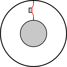
Suppose we have some current I flowing in a wire loop, as shown in figure 11.8. The current will gradually decay, on a timescale given by L/R, i.e. the inductance divided by the resistance.
The temperature of the wire will increase, and the entropy of the wire will increase, even though no energy is being transferred (thermally or otherwise) across the boundary of the system.
(Even if you consider an imaginary boundary between the conduction electrons and the rest of the metal, you cannot possibly use any notion of energy flowing across the boundary to explain the fact that both subsystems heat up.)
A decaying current of water in an annular trough can be used to make the same point.
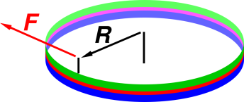
Here is a modified version of Rumford’s experiment, more suitable for quantitative analysis. Note that reference 31 carries out a similar analysis and reaches many of the same conclusions. Also note that this can be considered a macroscopic mechanical analog of the NMR τ2 process, where there is a change in entropy with no change in energy. See also figure 1.3.
Suppose we have an oil bearing as shown in figure 11.9. It consists of an upper plate and a lower plate, with a thin layer of oil between them. Each plate is a narrow annulus of radius R. The lower plate is held stationary. The upper plate rotates under the influence of a force F, applied via a handle as shown. The upper plate is kept coaxial with the lower plate by a force of constraint, not shown. The two forces combine to create a pure torque, τ = F/R. The applied torque τ is balanced in the long run by a frictional torque τ′; specifically
| ⟨ τ ⟩ = ⟨ τ′ ⟩ (11.2) |
where ⟨ … ⟩ denotes a time-average. As another way of saying the same thing, in the long run the upper plate settles down to a more-or-less steady velocity.
We arrange that the system as a whole is thermally insulated from the environment, to a sufficient approximation. This includes arranging that the handle is thermally insulating. In practice this isn’t difficult.
We also arrange that the plates are somewhat thermally insulating, so that heat in the oil doesn’t immediately leak into the plates.
Viscous dissipation in the oil causes the oil to heat up. To a good approximation this is the only form of dissipation we must consider.
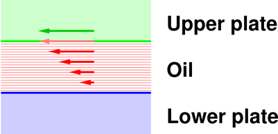
In an infinitesimal period of time, the handle moves through a distance dx or equivalently through an angle dθ = dx/R. We consider the driving force F to be a controlled variable. We consider θ to be an observable dependent variable. The relative motion of the plates sets up a steady shearing motion within the oil. We assume the oil forms a sufficiently thin layer and has sufficiently high viscosity that the flow is laminar (i.e. non-turbulent) everywhere. We say the fluid has a very low Reynolds number (but if you don’t know what that means, don’t worry about it). The point is that the velocity of the oil follows the simple pattern shown by the red arrows in figure 11.10.
The local work done on the handle by the driving force is w = Fdx or equivalently w = τdθ. This tells us how much energy is flowing across the boundary of the system. From now on we stop talking about work, and instead talk about energy, confident that energy is conserved.
We can keep track of the energy-content of the system by integrating the energy inputs. Similarly, given the initial entropy and the heat capacity of the materials, we can predict the entropy at all times1 by integrating equation 7.14. Also given the initial temperature and heat capacity, we can predict the temperature at all times by integrating equation 7.13. We can then measure the temperature and compare it with the prediction.
We can understand the situation in terms of equation 1.1. Energy τdθ comes in via the handle. This energy cannot be stored as potential energy within the system. This energy also cannot be stored as macroscopic or mesoscopic kinetic energy within the system, since at each point the velocity is essentially constant. By a process of elimination we conclude that this energy accumulates inside the system in microscopic form.
This gives us a reasonably complete description of the thermodynamics of the oil bearing.
This example is simple, but helps make a very important point. If you base your thermodynamics on wrong foundations, it will get wrong answers, including the misconceptions discussed in section 11.5.6 and section 11.5.7.
Some people who use wrong foundations try to hide from the resulting problems narrowing their definition of “thermodynamics” so severely that it has nothing to say – right or wrong – about dissipative systems. Making no predictions is a big improvement over making wrong predictions … but still it is a terrible price to pay. Real thermodynamics has tremendous power and generality. Real thermodynamics applies just fine to dissipative systems. See chapter 21 for more on this.
There are several correct ways of analyzing the oil-bearing system, one of which was presented in section 11.5.5. In addition, there are innumerably many incorrect ways of analyzing things. We cannot list all possible misconceptions, let alone discuss them all. However, it seems worthwhile to point out some of the most prevalent pitfalls.
You may have been taught to think of heating in terms of the “thermal” transfer of energy across a boundary. If you’re going to use that definition, you must keep in mind that it is not equivalent to the TdS definition. In other words, in section 17.1, definition #5 is sometimes very different from definition #2. The decaying current in section 11.5.4 and the oil-bearing example in section 11.5.5 clearly demonstrates this difference.
Among other things, this difference can be seen as another instance of boundary/interior inconsistency, as discussed in section 8.6. Specifically:
| No heat is flowing into the oil. The oil is hotter than its surroundings, so if there is any heat-flow at all, it flows outward from the oil. | The TdS/dt is strongly positive. The entropy of the oil is steadily increasing. |
Another point that can be made using this example is that the laws of thermodynamics apply just fine to dissipative systems. Viscous damping has a number of pedagogical advantages relative to (say) the sliding friction in Rumford’s cannon-boring experiment. It’s clear where the dissipation is occurring, and it’s clear that the dissipation does not prevent us from assigning a well-behaved temperature to each part of the apparatus. Viscous dissipation is more-or-less ideal in the sense that it does not depend on submicroscopic nonidealities such as the asperities that are commonly used to explain solid-on-solid sliding friction.
We now discuss some common misconceptions about work.
Work is susceptible to boundary/interior inconsistencies for some of the same reasons that heat is.
You may have been taught to think of work as an energy transfer across a boundary. That’s one of the definitions of work discussed in section 18.1. It’s often useful, and is harmless provided you don’t confuse it with the other definition, namely PdV.
| Work-flow is the “work” that shows up in the principle of virtual work (reference 32), e.g. when we want to calculate the force on the handle of the oil bearing. | Work-PdV is the “work” that shows up in the work/KE theorem. |
This discussion has shed some light on how equation 7.5 can and cannot be interpreted.
In all cases, the equation should not be considered the first law of thermodynamics, because it is inelegant and in every way inferior to a simple, direct statement of local conservation of energy.
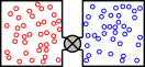
As shown in figure 11.11, suppose we have two moderate-sized containers connected by a valve. Initially the valve is closed. We fill one container with an ideal gas, and fill the other container with a different ideal gas, at the same temperature and pressure. When we open the valve, the gases will begin to mix. The temperature and pressure will remain unchanged, but there will be an irreversible increase in entropy. After mixing is complete, the molar entropy will have increased by Rln2.
As Gibbs observed,2 the Rln2 result is independent of the choice of gases, “… except that the gases which are mixed must be of different kinds. If we should bring into contact two masses of the same kind of gas, they would also mix, but there would be no increase of entropy”.
There is no way to explain this in terms of 19th-century physics. The explanation depends on quantum mechanics. It has to do with the fact that one helium atom is identical (absolutely totally identical) with another helium atom.
Also consider the following contrast:
| In figure 11.11, the pressure on both sides of the valve is the same. There is no net driving force. The process proceeds by diffusion, not by macroscopic flow. | This contrasts with the scenario where we have gas on one side of the partition, but vacuum on the other side. This is dramatically different, because in this scenario there is a perfectly good 17th-century dynamic (not thermodynamic) explanation for why the gas expands: there is a pressure difference, which drives a flow of fluid. |
| Entropy drives the process. There is no hope of extracting energy from the diffusive mixing process. | Energy drives the process. We could extract some of this energy by replacing the valve by a turbine. |
The timescale for free expansion is roughly L/c, where L is the size of the apparatus, and c is the speed of sound. The timescale for diffusion is slower by a huge factor, namely by a factor of L/λ, where λ is the mean free path in the gas.
Pedagogical note: The experiment in figure 11.11 is not very exciting to watch. Here’s an alternative: Put a drop or two of food coloring in a beaker of still water. The color will spread throughout the container, but only rather slowly. This allows students to visualize a process driven by entropy, not energy.Actually, it is likely that most of the color-spreading that you see is due to convection, not diffusion. To minimize convection, try putting the water in a tall, narrow glass cylinder, and putting it under a Bell jar to protect it from drafts. Then the spreading will take a very long time indeed.
Beware: Diffusion experiments of this sort are tremendously valuable if explained properly … but they are horribly vulnerable to misinterpretation if not explained properly, for reasons discussed in section 9.9.
For a discussion of the microscopic theory behind the Gibbs mixing experiments, see section 26.2.
It is possible to set up an experimental situation where there are a bunch of nuclei whose spins appear to be oriented completely at random, like a well-shuffled set of cards. However, if I let you in on the secret of how the system was prepared, you can, by using a certain sequence of Nuclear Magnetic Resonance (NMR) pulses, get all the spins to line up – evidently a very low-entropy configuration.
The trick is that there is a lot of information in the lattice surrounding the nuclei, something like 1023 bits of information. I don’t need to communicate all this information to you explicitly; I just need to let you in on the secret of how to use this information to untangle the spins.
The ramifications and implications of this are discussed in section 12.8.
Take a pot of ice water. Add energy to it via friction, à la Rumford, as described in section 11.5.3. The added energy will cause the ice to melt. The temperature of the ice water will not increase, not until all the ice is gone.
This illustrates the fact that temperature is not the same as thermal energy. It focuses our attention on the entropy. A gram of liquid water has more entropy than a gram of ice. So at any given temperature, a gram of water has more energy than a gram of ice.
The following experiment makes an interesting contrast.
Take an ideal gas acted upon by a piston. For simplicity, assume a nonrelativistic nondegenerate ideal gas, and assume the sample is small on the scale of kT/mg. Assume everything is thermally insulated, so that no energy enters or leaves the system via thermal conduction. Gently retract the piston, allowing the gas to expand. The gas cools as it expands. In the expanded state,
| Before the expansion, the energy in question (ΔE) was in microscopic Locrian form, within the gas. | After the expansion, this energy is in macroscopic non-Locrian form, within the mechanism that moves the piston. |
This scenario illustrates some of the differences between temperature and entropy, and some of the differences between energy and entropy.
Remember, the second law of thermodynamics says that the entropy obeys a local law of paraconservation. Be careful not to misquote this law.
| It doesn’t say that the temperature can’t decrease. It doesn’t say that the so-called “thermal energy” can’t decrease. | It says the entropy can’t decrease in any given region of space, except by flowing into adjacent regions. |
Energy is conserved. That is, it cannot increase or decrease except by flowing into adjacent regions. (You should not imagine that there is any law that says “thermal energy” by itself is conserved.)
If you gently push the piston back in, compressing the gas, the temperature will go back up.
Isentropic compression is an increase in temperature at constant entropy. Melting (section 11.8) is an increase in entropy at constant temperature. These are two radically different ways of increasing the energy.
Obtain (or construct) a simple magnetic compass. It is essentially a bar magnet that is free to pivot. Attach it to the middle of a board. By placing some small magnets elsewhere on the board, you should (with a little experimentation) be able to null out the earth’s field and any other stray fields, so that the needle rotates freely. If you don’t have convenient physical access to the needle, you can set it spinning using another magnet.
Note: The earth’s field is small, so it doesn’t take much to null it out. You can make your own not-very-strong magnets by starting with a piece of steel (perhaps a sewing pin) and magnetizing it.
Once you have a freely-moving needle, you can imagine that if it were smaller and more finely balanced, thermal agitation would cause it to rotate randomly back and forth forever.
Now hold another bar magnet close enough to ruin the free rotation, forcing the spinner to align with the imposed field.
This is a passable pedagogical model of the guts of a demagnetization refrigerator. Such devices are routinely used to produce exceedingly low temperatures, within a millionth of a degree of absolute zero. Copper nuclei can be used as the spinners.
The compass is not a perfect model of the copper nucleus, insofar as it has more than four states when it is spinning freely. However, if you use your imagination, you can pretend there are only four states. When a strong field is applied, only one of these states remains accessible.
It is worthwhile to compare theory to experiment:
| These values for the molar entropy s have a firm theoretical basis. They require little more than counting. We count microstates and apply the definition of entropy. Then we obtain Δs by simple subtraction. | Meanwhile, Δs can also obtained experimentally, by observing the classical macroscopic thermodynamic behavior of the refrigerator. |
Both ways of obtaining Δs give the same answer. What a coincidence! This answers the question about how to connect microscopic state-counting to macroscopic thermal behavior. The Shannon entropy is not merely analogous to the thermodynamic entropy; it is the thermodynamic entropy.
Spin entropy is discussed further in section 12.4.
Tangential remark: There are some efforts devoted to using demagnetization to produce refrigeration under conditions that are not quite so extreme; see e.g. reference 34.
As a practical technical matter, it is often possible to have a high degree of thermal insulation between some objects, while other objects are in vastly better thermal contact.
For example, if we push on an object using a thermally-insulating stick, we can transfer energy to the object, without transferring much entropy. In contrast, if we push on a hot object using a non-insulating stick, even though we impart energy to one or two of the object’s modes by pushing, the object could be losing energy overall, via thermal conduction through the stick.
Similarly, if you try to build a piece of thermodynamic apparatus, such as an automobile engine, it is essential that some parts reach thermal equilibrium reasonably quickly, and it is equally essential that other parts do not reach equilibrium on the same timescale.