Here are some notes concerning the book

This is just a collection of notes that I have accumulated. It should not be considered a book review. It is not by any means complete. Perhaps gradually it will become more complete and more balanced.

Note that a six-page list of known errata can be found in reference 1.

*   Contents

• 1  A Few Dozen Observations
• 2  Big Issues and Recurring Themes
  • 2.1  Limitations on the Range of Validity
  • 2.2  “Matter” versus “Interactions”
  • 2.3  Needless Radicalism and Needless Archaism
  • 2.4  Finite Differences versus Calculus
  • 2.5  Great Man Theory
  • 2.6  Field Lines, or Lack Thereof
    • 2.6.1  Virtually No Field Lines In the Book
    • 2.6.2  An Example of Field Lines
  • 2.7  The Topology of the Field is Important
    • 2.7.1  No Equipotentials, Either
    • 2.7.2  The AJP Article
  • 2.8  Vector Attachment
  • 2.9  Bogus Absolute Value Bars
  • 2.10  Regimentation Marches On
  • 2.11  Numbering the Equations
• 3  Bugs in the Index
• 4  Errors in the Errata
• 5  References

1  A Few Dozen Observations

Note that not all of these items are bugs; examples of non-bugs include item 12 and item 15.

1.

On the inside front cover, the periodic table shows La under Y, with an asterisk linking to the rest of the lanthanoids. It would be better to show a no single element under Y, just a blank space with an asterisk, and then to show the entire lanthanoid series in the inset. The entire series consists of 15 elements, from La to Lu inclusive. This is standard good practice, for excellent reasons. All theory and all data agree that La and Lu have an equally-good claim to sit directly under Y. It is important for students to see all 15 lanthanoids together. Ditto for the actinoids.

A lot of people who ought to know better think there should be 14 “f block” elements, but there is no data to support this. The set of integers from 0 through 14 inclusive has 15 members. People who cannot reliably count to 15 should not be telling other people how to do quantum mechanics. For details on this, see reference 2.

I realize this is not a major focus of the book, but it is one of those things where there is an upside to doing it right, and absolutely no downside.

2.

In physics, the traditional pedagogical sequence starts by describing the motion of particles that have no internal structure. Later, the laws of motion are applied to macroscopic objects, by treating the objects as collections of particles.

However, this book jumps directly into the deep end of the pool, making assertions about «objects». This evidently includes objects of every kind, large as well as small, non-rigid as well as rigid. This leads to lots of problems, because many of the assertions are simply not true when applied to extended objects (even though they would be true if applied to pointlike particles). For example:

• On page 6, it says that in the absence of interactions an «object» will exhibit «uniform motion». Alas that’s just not true for extended objects. In reality, a lopsided object does not generally exhibit uniform motion. For a hands-on example, see reference 3.
• On page 48, it says «No matter what system we choose, the Momentum Principle will correctly predict the behavior of the system.» I’m sorry, there’s a lot more to physics than F=dp/dt ... especially for extended objects.

3.

On page 5, there is a subsection about «An Object at Rest». The whole subsection violates Galileo’s principle of relativity. Just as there is no such thing as absolute motion, there is no such thing as absolute rest. You could say that two objects are at rest with respect to each other ... but you simply cannot say that either one of them is «at rest» in absolute terms.

The other subsections in this section are OK, because they use frame-independent concepts such as uniform motion and changes in velocity.

4.

On page 6, referring to the first law of motion, the book says «The English physicist Isaac Newton was the first person to state this law clearly. Newton’s first law of motion represented a major break with ancient tradition». The same idea is repeated on the next page.

In fact, though, Galileo clearly stated this law, many decades before Newton came on the scene. It was Galileo who made the major break with ancient tradition.

Imagine any particle projected along a horizontal plane without friction; then we know, from what has been more fully explained in the preceding pages, that this particle will move along this same plane with a motion which is uniform and perpetual, provided the plane has no limits. – Galileo Galilei (1638) tr. Crew & Salvio

It should also be noted that this law can be understood as a corollary of Galileo’s principle of relativity; see item 9.

We can give Newton credit for setting this law at the top of a numbered list, but that’s not the same as originating the law. See section 2.5 for more about this.

5.

Similarly, Newton was certainly not the first person to write F=ma. For starters, this is a highly modernized interpretation; it can perhaps be derived from what he wrote, but it’s not what he wrote – and other ways of interpreting what he wrote are arguably better. See item 73. Also note that F=ma is a vector equation, and vectors were not invented until hundreds of years later. See item 18 and also section 2.5.

6.

On page 9, it says in emphatic boldface: «Interactions cause change». I consider this to be bad pedagogy and wrong physics.

As to the physics, it is wrong coming and going:

• You could equally well say that interactions are responsible for the stability of ordinary terrestrial matter, i.e. the lack of change.
• On the other edge of the same sword, consider the superposition of two wave components, each of which is a standing wave, i.e. a stationary state. The superposition will be non-stationary. It will exhibit endless change, even though there is absolutely no «interaction» between the two components.

Perhaps more importantly, this depends on some profoundly incorrect assumptions about the role of «cause» and “effect” in the fundamental laws of physics, as discussed in reference 4.

As to the pedagogy, this is the sort of thing that leads to the worst sort of rote learning, because students think that if they learn those three words verbatim, they will be OK. In contrast, if they thought about those words at all, they would realize that they cannot possibly be true.

7.

The use of angle brackets ⟨⋯⟩ to express a vector in terms of components is highly nonstandard. Students will have to unlearn this. This is introduced on page 10 with no apology, with no explanation, indeed with no comment at all. It is then used throughout the book.

Every math and/or physics book I’ve ever seen uses square brackets for this purpose. M&I is my first exposure to angle brackets.

In particular, from the point of view of linear algebra, the sort of vectors we’re talking about are N×1 matrices. The things we call components are the matrix elements. For a matrix of any shape, everybody writes the matrix elements within square brackets. This includes N×M rectangular matrices, including special cases such as N×N square matrices and N×1 column vectors and 1×M row vectors.

8.

The book states on page 12 and summarizes on page 39 that it is «not legal (and not meaningful)» to add vectors to scalars, or to divide anything by a vector. This is grossly overstated, to say the least. For example, complex numbers are isomorphic to vectors in the plane, and it is routine to divide by such things, and to add real numbers to them. More generally, such operations are legal, meaningful, and routine in Clifford algebra (aka geometric algebra).

If you want to say such things are beyond the scope of the course, that’s OK ... but it is not helpful to say they are «not legal (and not meaningful)».

9.

On page 35, it highlights the «the principle of relativity». In the surrounding paragraphs, Galileo is not mentioned at all, whereas Newton is mentioned six times and Einstein once. This is quite unfair to Galileo.

Shut yourself up with some friend in the main cabin below decks on some large ship, and have with you there some flies, butterflies, and other small flying animals. Have a large bowl of water with some fish in it; hang up a bottle that empties drop by drop into a wide vessel beneath it. With the ship standing still, observe carefully how the little animals fly with equal speed to all sides of the cabin. The fish swim indifferently in all directions; the drops fall into the vessel beneath; and, in throwing something to your friend, you need throw it no more strongly in one direction than another, the distances being equal; jumping with your feet together, you pass equal spaces in every direction. When you have observed all these things carefully (though doubtless when the ship is standing still everything must happen in this way), have the ship proceed with any speed you like, so long as the motion is uniform and not fluctuating this way and that. You will discover not the least change in all the effects named, nor could you tell from any of them whether the ship was moving or standing still. In jumping, you will pass on the floor the same spaces as before, nor will you make larger jumps toward the stern than toward the prow even though the ship is moving quite rapidly, despite the fact that during the time that you are in the air the floor under you will be going in a direction opposite to your jump. In throwing something to your companion, you will need no more force to get it to him whether he is in the direction of the bow or the stern, with yourself situated opposite. The droplets will fall as before into the vessel beneath without dropping toward the stern, although while the drops are in the air the ship runs many spans. The fish in their water will swim toward the front of their bowl with no more effort than toward the back, and will go with equal ease to bait placed anywhere around the edges of the bowl. Finally the butterflies and flies will continue their flights indifferently toward every side, nor will it ever happen that they are concentrated toward the stern, as if tired out from keeping up with the course of the ship, from which they will have been separated during long intervals by keeping themselves in the air. And if smoke is made by burning some incense, it will be seen going up in the form of a little cloud, remaining still and moving no more toward one side than the other. The cause of all these correspondences of effects is the fact that the ship’s motion is common to all the things contained in it, and to the air also. That is why I said you should be below decks; for if this took place above in the open air, which would not follow the course of the ship, more or less noticeable differences would be seen in some of the effects noted. – Galileo Galilei (1638) tr. Drake

See also section 2.5.

10.

Beginning on page 37, the discussion of special relativity is problematic for several reasons.

For starters, it talks about «Einstein’s Special Theory of Relativity (published in 1905)». That is grotesquely misleading. Our understanding of relativity did not begin or end with Einstein, and it did not begin or end in 1905. There were major contributions from Galileo, FitzGerald, Lorentz, Poincaré, Michelson/Morley, Minkowski, and many many others. By far the most original and most consequential contributions were from Galileo (1638) and Minkowski (1908). See also section 2.5.

Let’s be clear: Our modern understanding of special relativity is based on contributions from many people, at least two of whom contributed far more than Einstein. Initially, Einstein downplayed Minkowski’s contribution, but before long he completely discarded the 1905 approach and relied on Minkowski’s spacetime approach for all later work, including General Relativity.

There is no excuse for sticking with the pre-1908 approach. It is more than 100 years out of date. It is more complicated, harder to explain, and harder to use. It must be completely unlearned before the modern approach can be learned. See reference 5.

11.

On page 37, the relativity section mentions that «time will run at different rates in different frames of reference». Alas that is inconsistent with any modern (post-1908) understanding of relativity. If you rotate a ruler, it does not change “the” length. By the same token, if you boost a clock, it does not change “the” time. See reference 5.

12.

Oddly enough, on page 38 the book uses a modern (post-1908) notion of mass, i.e. a velocity-independent definition of mass. I’m not complaining about this. I would rather see some modern concepts than none. However, it strikes me as odd that this would be combined with archaic velocity-dependent notions of time and distance.

13.

On page 38, section 1.11 starts by saying the velocity is approximately p/m. Then equation 38.65 says:

« |p→|   =   1 √ 1−(v/c)2  m |v→| »              (1)

That’s not exactly wrong, but it is unreasonable, because it is far messier and uglier than it needs to be. By “not exactly wrong” I mean that the correct physics is a solution to the equation; however, there are also innumerable unphysical situations that also satisfy the equation. We should contrast it with the modern (post-1908) way of expressing the same idea, namely

p   =   m u

(2)

where p and u are four-vectors.¹ This equation could hardly be simpler. Compared to equation 1, it is easier to understand, easier to explain, and easier to use.

For starters, the absolute-value bars in equation 1 are silly. They’re not exactly wrong, but they make the equation more complicated, less trustworthy, and less useful.

Note that the «p→» that appears in equation 1 is not the quite the same as the p that appears in equation 2. In fact «p→» is the projection of the four-dimensional momentum p onto the spatial directions xyz in some chosen frame. It would be better to write the LHS of equation 1 in terms of p_xyz or something like that ... and even better to forget about equation 1 and write equation 2 instead.

The p that appears on the LHS of equation 2 is the full four-dimensional momentum. Similarly, the u on the RHS is the full four-dimensional velocity. As discussed in reference 5, it is defined as:

u   :=   dx dτ

(3)

where x is the full four-dimensional position vector, and τ is the proper time. This equation could hardly be simpler. It is simple in its structure and simple in its conceptual interpretation.

The inverse square root that appears in equation 1 is best understood as a factor of dt/dτ, which results from choosing an unfortunate way of measuring time. The proper time τ makes things simple. The coordinate time t is the projection of τ onto some chosen basis, and it makes things seem more complicated than they really are, for instance when it is used to calculate the reduced velocity v that appears in equation 1. For details, see reference 5.

14.

On page 41 in 1.X.52 it refers to a «Bernoulli blower». This is a misnomer. The device in question has got nothing to do with Bernoulli, in much the same way that a platinum AMEX card does not contain real platinum.

This appears to be the only mention of Bernoulli in the whole book.

Suggestion: Just describe the physics, without the misleading name. A ball is suspended in a jet of air, i.e. in a narrow fast-moving stream of air.

15.

In question 1.X.32 on page 24 and in the answer on page 47, there is a golden teachable moment. The lesson is check your work. There are at least four ways of obtaining the answer to this question. Students should be required to carry out at least two of them (preferably three or four) and check for consistency.

The check-your-work rule is the cornerstone of critical thinking.

In later chapters, the check-your-work rule should go without saying, but here in chapter 1 it would be nice to mention it explicitly.

16.

On page 49, it says force is «the cause» and change in momentum is «the effect». This has no basis in physics and is inconsistent with fundamental notions of cause and effect, as explained in detail in reference 4. Compare item 30.

17.

On page 49, the Momentum Principle is introduced as Δp = F_net Δt ... even though it would be more correct to write it as dp = F_net dt.

As discussed in section 2.4, I understand that at this point in the course, there are reasonable reasons for avoiding calculus concepts and calculus notation.

I would like to make a different point, focusing on the words that talk about the equation. The book highlights «the momentum principle» and bills it as a «fundamental principle» that «applies to every possible system» ... even though the formula as stated is not correct in general. It’s hardly even meaningful unless we assume that the force is constant, which is not the general case.

Suggestion: It would be better to say something to the effect that a more precise statement of the momentum principle will be given later, implicitly on page 125 and explicitly in equation 155.22. This a manifestation of the “limitations” issue, as discussed in section 2.1.

18.

Throughout the book, the formula F=dp/dt is wrongly named «the momentum principle». This is not a brilliant innovation; it’s just weird. There are at least three reasons why this makes no sense:

• By far the most important “momentum principle” is conservation of momentum. Since the book uses the term “energy principle” to refer to conservation of energy, it seems astonishingly illogical and inconsistent to use «momentum principle» to refer to anything other than conservation of momentum ... especially given that energy and momentum are part of the same four-vector.

  Pretending there is only one momentum-related principle cannot be justified on any scientific or pedagogical grounds. Students who learn this weird terminology will be at a handicap when trying to communicate with the rest of the population.

• I remark in passing that momentum appears on one side of the equation and force on the other, so it would make at least as much sense to call it “the force principle”.
• On top of all that: The equation F=dp/dt already has a name: It is known as the second law of motion ... and has been since Day One.

  LEX II. Mutationem motus proportionalem esse vi motrici impressæ, & fieri secundum lineam rectam qua vis illa imprimitur. – Isaac Newton (1687)

Similar remarks apply to «the angular momentum principle» on page 426 and elsewhere. Contrast this with item 36.

19.

The definition of g on page 66 is inconsistent with the definition on page 101.

Suggestion: The LHS of the law of universal gravitation really needs to be written as δg_m. It is two jumps removed from the gravitational acceleration g. In the usual terrestrial lab frame, δg_m is the largest single contribution to g, but it is not the whole story. See the discussion of “various different notions of gravity” in reference 7.

20.

On page 66, we find a definition of «our usual reference frame». The y axis is defined relative to the earth, while the z axis is defined relative to the book. In the exceedingly common case where the book is lying flat on a horizontal surface, this definition makes no sense.

Furthermore, it must be emphasized that when the book speaks of «our» usual reference frame, the authors are speaking only for themselves, not for the larger community. Throughout the physics and engineering literature, if there is a vertical axis, the near-universal choice is to call it the z axis.

21.

On page 71, the instructions for «checking that Δt is small enough» are not reliably correct. Sometimes an inaccurate result is obtained because the step-size is too small – not too large. This can easily arise due to accumulation of roundoff errors.

22.

On page 71 and especially on page 105, the equations do not match the words or the diagrams. In particular, consider equation 71.18, namely «p_f = p_i + F[net]Δt». By reverse-engineering the numerical examples, we can infer that the intended meaning is p_f = p_i + F[net]_iΔt, where I have added a subscript i to F[net], to indicate that force is to be evaluated at the beginning of the step. However, on the very next line we find equation 71.22, namely «r_f = r_i + v[avg]Δt where v[avg] ≈ p_f/m». That seems to say the velocity is to be evaluated at the end of the step.

• One way of looking at this is to call it an abuse of the notion of “average”. The update rule for the position uses the “average” velocity, averaged over the whole step-1 interval, while the update rule for the momentum uses the “average” force in the neighborhood of the step-0 / step-1 boundary, which is not a reasonable estimate of the “average” over the actual interval being considered, i.e. the interval shown in the diagram.
• Another way of looking at it is as an example of equation hunting. “Some” kind of force is plugged into the equation «p_f = p_i + F[net]Δt», but it is not the appropriate force, not compatible with the originally-defined meaning of the equation.
• Yet another way of looking at it is to call it an abuse of the symbols, including Δ, i (for initial) and f (for final). These symbols are being used in inconsistent ways. For example, r_i and r_f refer to the “initial” and “final” positions, at the beginning and end of the step-1 interval. In contrast, p_i and p_f do not have any similar interpretation. There are various ways to fix this, for instance by recognizing that for practical purposes the momentum update is happening at a single point – at the boundary between steps – and defining p_b and p_a, where the subscripts b and a stand for “before” and “after”, namely before and after the the step-0 / step-1 boundary. Another way to fix it would be to define a staggered step, consisting of the last half of step 0 and the first half of step 1.

  This illustrates the distinction between calculus and finite-difference methods. As discussed in section 2.4, the inconsistencies would go away if we were using calculus i.e. passing to the limit as Δ goes to zero. However, computers operate on finite differences, and the inconsistences affect how the code is written, and can dramatically affect the results.

If you want the students to learn by rote to write the code a certain way, that would be semi-OK ... but please let’s be upfront about it. Let’s not pretend that the code is explained by the physics, when the real explanation has not been given. Conversely, if you want the students to understand what’s going on, you have to give the actual explanation.

Let’s be clear: Suppose a student understood the diagrams and understood the words in the text – words like “step” and “average” – and wrote some code accordingly. This student would get a very much worse result than a student who wrote the code in rote obedience to the recipe outlined in the text. Neither student would understand why, and in all likelihood the teacher wouldn’t either.

The explanation is that one approach results in a symplectic integrator, while the other does not; see reference 8. There is no way to explain this in terms of the “average” force or “average” velocity, averaged over some “step”.

23.

On page 81, in the margin box, there is an argument in terms of units that would be vastly better in terms of dimensions. See reference 9.

24.

On page 102 it equates «up» with the direction «away from the center of the Earth». This is not entirely correct; see item 54 and reference 7.

25.

Also on page 102 it says that «g is smaller at the equator», which is true, but alas it attempts to explain that by saying «you’re farther from the center of the earth». In reality, g is less at the equator by about 0.5%, and the centrifugal field explains most of this, about 0.3%, leaving about 0.2% to be explained by the distance from the center. Alas, a simple calculation based on the square of the radii predicts 0.67% from this factor alone, which is dramatically larger than the right answer of 0.2%. The gravitational physics here is fundamentally wrong. Part of the problem comes from considering only mass and distance, which works OK for spherical distributions but not for anything else, in particular not for ellipsoids.

This is on top of the even more obvious fundamental error of disregarding the centrifugal field; see also item 32.

For the correct physics of hydrostatic shapes and surface gravity, see reference 10.

26.

On page 103, the term «reciprocity» is featured.

The book all-too-consistently uses reciprocity as a code-word to refer to the third law of motion. This is not helpful. All the world refers to the third law as the third law. Furthermore, in physics, recprocity already has a well-defined technical meaning.

27.

Perhaps even more seriously, the discussion on page 103 connects the third law (aka «reciprocity») to electrostatics and gravitation. There is not the slightest hint that the law might apply more generally than that.

It is important to get this right, because the third law is tantamount to conservation of momentum. There could hardly be anything more important.

28.

On page 117, the symbol Δ presumably refers to the standard deviation of some probability distribution. This is inconsistent with how the symbol is used almost everywhere else in the book ... as exemplified by the emphatic reminder on page 665.

29.

On page 163, the numbers for the composition of the atmosphere are unnecessarily rough. There is no good reason why 78.09% should be rounded off to 80. Also, it’s just not true that all the other gases are present in «very small amounts».

At the very least, the numbers should be specified as applying to dry air.

Dry air contains roughly 78.09% (by volume) nitrogen, 20.95% oxygen, and 0.93% argon. In addition, there can easily be several percent of water vapor mixed in.

30.

On page 197, there are three paragraphs in the section entitled «F_net and dp/dt Are NOT the Same!». The first two paragraphs correctly describe the symmetrical relationship: If you know F you can calculate dp/dt and vice versa. To this I might add that in the second law of motion, both sides of the equation (F = dp/dt) are functions of time, and both sides are evaluated at the same time. The only problem with these two paragraphs is that they do not support the nominal topic of the section; they do not contribute toward explaining the distinction between force and dp/dt.

Alas the third paragraph in this section is profoundly wrong. For starters, we can tell that it is wrong because it contradicts the previous two paragraphs, insofar as it alleges an asymmetrical relationship between F and dp/dt. Furthermore, it is proof by bold assertion, with absolutely no evidence to back it up. The asymmetrical relationship is symbolized by an arrow, and also analogized to the highly asymmetrical relationship between cause and effect. Note that according to the usual definitions, a cause must precede its effect, so this breaks the equal-time property of the second law (in addition to breaking the symmetry).

For more about cause-and-effect and its relationship to the basic laws of physics, see reference 4. Compare item 16.

31.

Perhaps more importantly, we should consider what has not been said about the status of the second law. The key idea is to distinguish an equality from a tautology. Specifically:

Traditionally, physics has not defined force in terms of momentum (or vice versa), but rather has used independent operational definitions of these quantities. Therefore the second law is not a tautology. It tells us something we did not already know.

In principle, I suppose one could define force in terms of dp/dt, in which case we would have a tautology. The book comes rather close to doing this ... so close that the denial on page 197 was deemed necessary.

This highlights the fact that the book does not do a very good job of laying down a solid operational definition of force ... unless I have overlooked something, something that is not mentioned in the index or the table of contents. This stands in contrast with PSSC Physics which in my opinion does an outstanding job of defining force in terms of a standard spring. It goes on to give a simple yet scrupulously principled explanation of the algebraic properties that a force must have.

To say the same thing another way, when page 197 says «F_net and dp/dt Are NOT the Same!», that is non-constructive. It tells us what the relationship isn’t ... whereas it would be much more constructive to tell us what the relationship is.

32.

On page 200, figure 5.41(b) and the associated discussion indicate that centrifugal force is «incorrect».

However, the fact is that the centrifugal field is as real as the ordinary laboratory gravitational field. Both are 100% dependent on choosing a non-inertial reference frame. In particular, the centrifugal field exists in the rotating frame and not otherwise. See reference 11 for a discussion of how this works.

This contributes to getting the wrong answer in item 25.

This is particularly relevant, because people tend to identify with people, and the book presents example after example where real-world people would not naturally use the terrestrial laboratory frame, namely the people aboard the orbiting space station, the person swinging on the vine, the people aboard the airliner, the people riding the Hoffmeister rotor, et cetera. On page 203 it quite explicitly focuses on the «feeling» of the passengers. In all these situations, real-world people would be entirely within their rights to choose a rotating reference frame in which centrifugal forces are key to analyzing the situation.

It would be OK to say that rotating reference frames are outside the scope of the course ... but it is absolutely not OK to suggest that they don’t exist or are «incorrect». See reference 11.

The thing that really cracks me up is the utter futility of saying that the rotating-frame analysis is wrong. Based on years of experience such as riding in cars, students can tell by the seat of their pants – literally – that the centrifugal field exists. Even if you train them by rote to say in class that the concept of centrifugal force is wrong, as soon as they step outside the classroom they will go back to using the concept ... probably using it more-or-less correctly.

See also section 2.10.

33.

As a related point, on page 203 and page 204 there is a discussion of weightlessness, including a sidebar that mentions General Relativity. Alas, however, what is said about weightlessness is completely backwards from the General Relativity point of view. It puts «“weightless”» in scare quotes, for no good reason. You can’t have it both ways. You can either take a 17th-century view of the situation, or you can invoke General Relativity, but you can’t do both. See reference 7.

34.

On page 215 in 5.P.56, we find the same untenable view of weight and weightlessness. It is perfectly OK to define “weight” in terms of the gravitational force Mg; the problem is upstream from there, in the definition of g itself. The definition of g simply must be frame-dependent. We could figure this out using modern physics, namely Einstein’s principle of equivalence, but we can also figure it out based on prosaic, classical, operational considerations. The laboratory value of g simply must include contributions from the motion of the reference frame, namely the rotation of the earth; otherwise basic notions of “horizontal” and “vertical” would be noticeably incorrect. See reference 7.

35.

On page 215 in 5.P.56, the speculation about «internal organs» and «the odd sensation in your stomach» is not correct. Note that lying down greatly modifies the stress on the internal organs, but does not produce the same sensation. In fact, nausea originates in the inner ear and in the brain. In turn, the brain may (or may not) do odd things to the stomach. Evidence for this includes the fact that training matters: experience with roller coasters, swings, and/or aerobatic aircraft makes the «odd sensation» go away.

36.

Throughout the book, especially in chapter 6 (starting on page 220), conservation of energy is wrongly named «the energy principle». This is a serious problem, because there are lots of principles that involve energy. Conservation is the most important one, but not the only one.

Also note that this is inconsistent with the definition of «the momentum principle», as discussed in item 18.

Further note that on page 118, conservation of momentum is called «conservation of momentum». Similarly on page 585, conservation of charge is called «conservation of charge». This suggests that there cannot be any principled reason why conservation of energy could not be called by its proper name.

37.

In the long discussion beginning on page 226, there is, alas, no explanation of the distinction between work done by a system and work done on a system. It appears the book defines W to be positive when work is done on “the” system by some external force. However, this is not a sufficient explanation, because it leaves plenty of situations where the sign of W is not at all obvious. The problem is not with the definition of W, but instead is farther upstream, in the definition of “system”. For example:

• If one student pushes another, is this positive work or negative work? It depends on which student you consider “the” system. Symmetry tells us the question is unanswerable, as a matter of principle.
• If you catch a fastball, is this positive work or negative work? You could say negative work is done on the ball by you ... or you could say positive work is done on you by the ball.

If one is not fastidious about the work-by/work-on distinction, all sorts of minus-sign errors show up. Errors affecting the sign of W can be found in the text; see section 4 and item 76.

The non-coverage of this issue is particularly glaring when contrasted with the amount of attention given to less-important issues in this section, e.g. in the subsection «Positive and Negative Work», the subsection «A Common Mistake», and the subsection «Sign of Work Depends on Direction of Force and Direction of Motion».

This issue is exacerbated by the fact that most of the thermodynamics literature adopts the opposite convention, using W to represent the work done by the engine, for obvious reasons. This means the students are likely to be confused the first time they read anything other than this book.

Tangential remark: This touches on an even deeper fundamental issue: Introductory texts tend to talk in terms of “the” system and “the” surroundings. This is unworkable in the long run. It breaks down in some quite simple systems; for instance, when one student pushes on another, symmetry makes it impossible to decide which student is the “system” and which is the “surroundings”. The breakdown is even more spectacular in more complicated situations, such as in fluid dynamics, where one must divide the fluid into many parcels, each of which acts as a “system” unto itself, even while acting as part of the “surroundings” for other parcels.

Suggestion: Be painstakingly explicit. Rather than writing simply W, write W[on gas] or W[by engine] or whatever.

38.

Another suggestion: In general, it is best to avoid the symbol W altogether, and instead write a longer expression such as F·dx or −PdV. Also avoid Q altogether, and instead write TdS. There are eleventeen strong reasons for this, not least the fact that W and Q as used in the text are not functions of state, but rather functionals of the path, depending on every detail of the path from initial state to final state ... and students at this stage have not the slightest idea what a functional is. In contrast, F·dx, PdV, and TdS are perfectly fine functions of state. They’re not scalars, but they are functions of state. For details on how this all works, see reference 12.

As further evidence for the importance of this, consider the endless holy wars over the definition of “heat” that one finds in the PER literature.

39.

On page 241, equation 241.13 is billed as the «general definition of work», namely

« W   ≡   ∫ f i  F·dr »

(4)

On page 527, equation 527.77 expresses the same general idea:

« W   =   − ∫ V2 V1  P dV »

(5)

Equation 527.77 appears in a section that focuses attention on an isothermal compression, so no harm would be done if the student wrote this restriction next to the equation, explicitly:

W   =   − ∫ V2 V1  P dV      at constant temperature

(6)

Equation 528.69 expresses the same idea:

W   =   − ∫ V2 V1  P dV      at constant temperature

(7)

The same symbols appear again in equation 530.26 ... but with a different meaning:

W   =   − ∫ V2 V1  P dV      at constant pressure

(8)

The same symbols appear again in equation 531.07, with yet a different meaning:

W   =   − ∫ V2 V1  P dV      at constant entropy

(9)

At this point the student will almost inevitably conclude that the unadorned equation 5 is true in general, without restriction. Evidently it was a waste of time to keep track of the limitations as shown in magenta above. The only problem is, equation 5 is not true in general! Equation 4 is not the «general» definition of work. Somebody with a solid understanding of thermodynamics would know this, but the student has no way of figuring this out.

Keep in mind that at this point in the course, the student might have studied calculus for only about half a year. According to everything we know about calculus at this level (and several levels beyond that), the RHS of equation 5 implicitly demands that the LHS be considered a function of V₁ and V₂. We can make this explicit by rewriting it as:

W(V1, V2)   =   − ∫ V2 V1  P dV      ☠

(10)

The problem is, equation 10 is grossly incorrect (when applied to uncramped thermodynamics). In particular, consider a complete thermodynamic cycle, in which the initial state (1) is the same as the final state (2). Equation 10 tells us that the work done by any thermodynamic cycle is zero. There is no other reasonable interpretation of this equation.

In order to understand thermodynamics we need to treat W as a functional of the entire path Γ that connects state 1 to state 2. Someone with a solid understanding of thermodynamics would write it as

W[Γ]   =   − ∫   Γ  P dV

(11)

Alas, the chance that students will figure this out on their own is virtually zero. This concept needs to be explained. Indeed it will take a lot of explaining, especially if they have never seen the concept of “functional” before, or even so much as heard the word.

Equation 5 is an impediment to understanding, because it indicates to the student that W is something it’s not. This is a conspicuous example of the “limitations” issue discussed in section 2.1.

This problem is further exacerbated by negative transference of the following kind: Students come to class with years of experience – and years of schooling – restricted to cramped thermodynamics, i.e. situations so restricted that it is impossible in principle to build a heat engine. Specifically, I’m talking about situations like warming a bottle of milk and then cooling it off again, i.e. situations where the heating and cooling are restricted to a single one-dimensional simply-connected path through thermodynamic state space. In cramped situations, you can get away with using equation 5 and similar equations that suggest that heat-content and work-content are functions of state. Students more-or-less universally assume that these equations are valid in general, which is a tremendous barrier to understanding.

Telling the students once or twice that heat-content (aka caloric) is not a function of state is nowhere near sufficient. They need a workable set of modern concepts to replace their 18th-century notion of caloric. Things like equation 5 are exactly what they do not need. Equation 11 is correct but difficult for students to understand. My point is that that replacing a difficult equation with an incorrect equation is not helpful. For details on how to do this right, see reference 12.

40.

On page 270 it says «Since the momentum required to touch is less than the momentum required to initiate the reaction, the reaction can in fact occur.» Sorry, that is nowhere near being the criterion for whether a reaction can occur. I have no idea what this is trying to say.

41.

Consider the following statements:

1. On pages 301–302, «heat» is defined as «Q = energy transfer due to a temperature difference».
2. On page 303, this same Q is used in the alleged statement of «the energy principle».
3. On page 483, we find the «definition of entropy S».
4. On page 487, we find the «definition of temperature T» in terms of entropy and energy.
5. On page 488, we find the «entropy change associated with small Q», namely

   ΔS   =   Q T

   (12)

There is a serious inconsistency somewhere here. You could arrange to make any one of those statements true, and maybe even two or three of them, but not all of them at the same time.

Consider a situation where Q is zero, in the sense of page 301, i.e. no thermal transfer of energy. If we plug this same Q into equation 12, we find that ΔS must be zero (assuming nonzero temperature). In other words, the entropy must be constant. However, we know that’s not true, because there are lots of ways that entropy can increase without being transferred across a boundary. The falling coffee filters on page 311 are an example. The case of a block rubbing against an identical block is an example where it is even more obvious that no «heat» is being transferred, even though the entropy is increasing. It’s obvious by symmetry.

The fundamental problem is that in physics, there are multiple inconsistent definitions of «heat». The book gives one of the definitions on pages 301–302, but then mixes in the others without warning, without explanation.

The simplest way out of this mess is to explain that the ΔS in equation 12 is only one contribution to the total change in entropy. There are other contributions as well. This is quite a significant statement, especially given that in classical (pre-1898) thermodynamics, equation 12 was used to define entropy.

For more perspective on this mess and how to avoid it, see reference 12.

42.

Starting on page 302, «thermal energy» and E_thermal are mentioned several times.

In any uncramped situation, i.e. in any situation where it is possible in principle to build a heat engine, it is provably impossible to define a state function that quantifies the «thermal energy». Calling it «thermal energy» instead of “heat” or “caloric” does not help, not even a little bit. For example, suppose I have one liter of nitrogen gas at STP. How much «thermal energy» does it contain? How much nonthermal energy? I have no idea how much, because the question is ill-posed.

Everything that chapter 7 (“Internal Energy”) says about «thermal energy» content will have to be unlearned as a prerequisite for getting through chapter 13 (“Gases and Engines”).

43.

On page 304, even after errata are applied (i.e. as of 5th printing), standard math notation does not define anything like

F • dr dt

On the previous line in the text, Δy/Δx is indeed a fraction, and obeys the usual rules for fractions.

However, dy/dx is pronounced “dx by dy” not “dx over dy” and is not really a fraction. It is written in a way that looks like a fraction, but technically it is not dy divided by dx. The only thing dy by itself could possibly refer to is the exterior derivative, and dy/dx is not the ratio of two exterior derivatives. It is best to consider dy/dx as an invariable idiomatic expression. It doesn’t really have a numerator or a denominator, so it doesn’t make sense to stick “F” in the supposed numerator.

Specifically, rather than

power =  F • Δr Δt      power =  F • dr dt = F •  dr dt = F•v                (13)

it would be better to factor out the F before passing to the limit of Δ→0.

power =  F • Δr Δt = F •  Δr Δt      power t = F •  dr dt = F•v                (14)

The same issue arises again at the top of page 305.

44.

On page 316 it introduces the term «nonconservative». This is a misnomer. It is practically begging to be misunderstood. I recommend “non-grady” instead, to denote something that is not the gradient of any potential. See reference 13.

45.

On page 316 it confuses the idea of «dissipative» with «nonconservative».

Counterexample: betatron. See reference 13.

46.

On page 322 in item 7.P.47(a), it would be better to speak of energy consumption. One does not consume power. The dimensions are wrong.

47.

On page 326 the term «photon» is defined.

Alas, there are two inequivalent definitions of photon in common use in the physics community. The definition given here is not wrong, but it is not the whole story.

1. A photon is an excitation of a particular mode of the EM field. Each mode of the field is a harmonic oscillator, and as such the energy states are quantized, and the quantum number N is called the photon number.

   Any such photon is necessarily monochromatic.

2. A photon is a localized wave packet. Typically one imagines a Gaussian envelope on top of a running-wave carrier.

   Any such photon is necessarily not monochromatic. If it is localized, it can’t be monochromatic.

48.

On page 326 it restricts the application of quantum ideas to «microscopic systems». The same idea is repeated many times in the pages that follow. This is not consistent with a modern understanding of physics. As far as we can tell, there is only one set of physical laws. The laws of QM apply to everything, large and small. The laws of QM tell us when the classical approximation is valid. (The converse, however, does not not hold: Classical physics cannot tell us very much about QM.)

Note that there are many macroscopic systems where quantum effects play a prominent role. See e.g. reference 14.

49.

On page 326 it says «The internal energy of microscopic systems is quantized; that is, the internal energy of the system can have only certain specific values (“energy levels”). The system is never observed to have energies between these levels.»

That’s either wrong or highly misleading. It is in fact routine to find systems in states that do not correspond to any of the quantized “energy levels”.

For starters, every sinusoidal voltage you’ve ever seen – and the sinusoidal motion of every oscillator you’ve ever seen – corresponds to a coherent state, not a definite-energy state. For more about coherent states, see reference 15.

As another example, every atomic transition has some nonzero linewidth. This tells us that every state (except possibly the ground state) corresponds to a range of energies.

Similar words apply to quantization of angular momentum; see item 56.

50.

On page 383, it says «Neglecting external interactions allows us to apply both the Momentum Principle and the Energy Principle in their strongest forms: Conservation of Momentum and Conservation of Energy.» The energy part of that is inconsistent, because the «Energy Principle» was defined to be conservation of energy, and there are not, so far as I know, any stronger or weaker forms of this. Energy is conserved, period.

Meanwhile, the momentum part of this is exceedingly weird. It’s like saying the black eagle shrieked at dawn, and therefore we can use conservation of momentum. My point is that that momentum is always conserved, period. There is no need for any shaggy dog stories or any other preconditions for applying conservation of momentum.

I assume a major purpose of the course is to teach students to think clearly. This exceedingly muddled reasoning is unhelpful. See also item 18.

51.

On page 386, figure 10.5 shows the figure shows the final position of cart 1 being equal to the initial position of cart 2, which is quite wrong. It’s off by an entire cart-length. In fact cart 1 takes over the velocity of cart 2, but not the position.

52.

On page 383, it talks about «“Collisions” without Contact». Certainly such a thing is possible, but the two examples that are given are the most inappropriate examples possible. The Coulomb scattering between an electron and a proton is an infinite-range interaction. For details on what I mean by that, see e.g. reference 16. It’s not at all clear that infinite-range scattering is covered by the «definition of collision» given on page 382.

Similarly, the «gravitational interaction of two asteroids» is an infinite-range interaction.

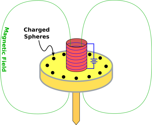
Suggestion: Choose some better examples, such as a small iron ball being scattered by the magnetic field in the gap of a large magnet, such as the one shown in figure 6. Given suitable initial conditions, the ball is deflected, even though it does not hit the pole pieces or any other part of the magnet. With skill you can arrange that it des a loop-de-loop and then emerges without being captured, such that the ball’s momentum vector rotates by slightly more than 360 degrees.

53.

On page 434, the velocity field of a rigid disk should be divergence free. This is not the least bit obvious from the diagram, because of the style in which the vectors are diagrammed. See section 2.8.

54.

Also on page 434, it says that on Earth, «gravitational forces act on it effectively through its center». That’s not exactly true. Most people do not have a good way of determining the direction from their location to the center of the earth ... but if they did, they would find that it is significantly different from the direction of the local gravitational field, at temperate latitudes. If you built a tall building aligned with the direction toward the center of the earth, it would be quite noticeably non-vertical. If you built a swimming pool aligned perpendicular to the direction toward the center of the earth, it would be quite noticeably non-horizontal. The pool would be tilted relative to the water. For details on this, see reference 7.

In the next paragraph it mentions the equatorial bulge, and mentions tides, and says that «over many thousands of years» these can lead to noticeable effects. I suppose that is true as far as it goes, but it is nowhere near being a sufficient correction to the errors in the previous paragraph. An accurate map is all you need to detect that gravity does not point toward the center of the earth; you do not need to wait thousands of years. See reference 7.

Similar errors are discussed in item 24.

55.

Starting on page 443, there is a multi-page discussion of the Bohr model of the atom, including diagrams of electrons going around the nucleus in circular orbits ... not quantum-mechanical orbitals, but actual orbits! With quantized radii!

When the Bohr model was first proposed, 100 years ago, it was better than all competing models. However, for 85 of those 100 years, the Bohr model has been out of date. There is no good reason to mention it at all. Much better models are available. Everything in this section will have to be unlearned as a prerequisite to understanding anything useful about quantum mechanics in general or atoms in particular.

Suggestion: If you feel the urge to talk about the Bohr model, lie down until the feeling goes away.

Of course it is important to have “some” model of how atoms work, but it would be a tremendous mistake to think there is a choice between the Bohr model and nothing ... or between the Bohr model and some prohibitively complex alternative.

Constructive suggestions include:

1. Perhaps the best advice is to get a circular tub or pool of water and practice setting up various wavefunctions.
2. You can also study waves on a string, which is a good model for shedding light on some of the things that atomic wavefunctions do.
3. There are also computer models that use dot-density animations.
4. There are also computer models that use color-coded phase and amplitude.
5. If you feel obliged to mention the constant known as the Bohr radius, you could derive it using a particle-in-a-box argument. See e.g. Feynman volume III page 2-6. The effort involved for writing down the particle-in-a-box wavefunctions is less than for writing down the circular Bohr orbits. It is no less correct, and is incomparably better as a foundation for further developments.
6. Instead (or additionally), you could model the atom as a harmonic oscillator, i.e. as a charged mass on a spring. Then talk about the states of a quantum harmonic oscillator. Once again, this would be far better than the Bohr model as a foundation for further developments (including phonons, photons, et cetera). Also, this would be very much more in line with everything else in the book, starting with the iconic ball-and-spring model on the cover.
7. Et cetera.

Several of these suggestions are discussed in more detail in reference 17.

The Bohr model doesn’t explain anything ... not anything worth knowing anyway. It successfully predicts a hydrogen energy spectrum that agrees with experiment, but this agreement is essentially fortuitous. Specifically, there is nothing in the Bohr model to explain why makes some correct predictions for a 1/r potential, and for nothing else. If you apply the Bohr model to 92 different elements, you get more than 91 incorrect predictions. Even for hydrogen, it gets the wrong answer for the angular momentum of the ground state. It also gets the optical selection rules all wrong.

It seems like a poor use of resources to focus attention on the Bohr model, to the exclusion of other models that are simultaneously simpler and more informative.

56.

Also on page 443, it says that angular momentum «is quantized». Alas, that’s not always true. Angular momentum is not any more quantized than energy is. If you happen to put the atom into a state of definite angular momentum, then the angular momentum is quantized, but if you don’t it isn’t. Compare item 49. For more on this, see reference 15.

57.

On page 475 it says «As predicted by quantum mechanics and abundantly confirmed by experiments, energy can be added to a one-dimensional atomic oscillator only in multiples of one “quantum” of energy ℏω₀»

Sorry, no, that is neither predicted by quantum-mechanical theory nor confirmed by experiment. Just the opposite. See e.g. reference 15.

This issue has been discussed since Day One of quantum mechanics. Planck used quantization of energy as an Ansatz, as a hypothesis. The fact that it led to a formula that was consistent with experiment does not prove that the hypothesis is correct, nor does it rule out the possibility that other hypotheses would lead to the same formula. Planck was well aware of this, and emphasized the point. A lot of people thought he was being overly cautious, but it turns out he was completely right. Energy is not necessarily quantized, and there are lots of other ways of getting the correct black-body radiation formula.

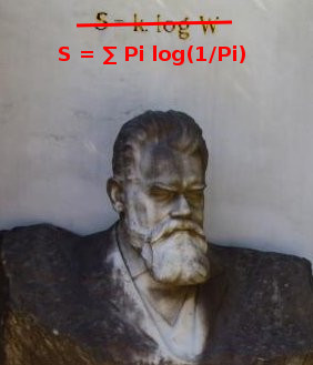
The most general expression for the entropy is the quantum statistical mechanics expression

S   =   − Tr ρ log ρ

(15)

which gives the same result in any basis. The energy-eigenstate basis is no worse than any other basis, but it is no better. In Planck’s day the formalism was nowhere near capable of expressing this result clearly, but it is now. The result is sensitive to the number of states in the basis, but not to which basis you use. The number of states is unchanged by a change of basis.

As I have said before:

Energy states are not the only states. They are not even the only basis states.

Suggestion: Rather than falsely saying that the energy is quantized, it would be better to say that statistical mechanics requires us to be able to count how many basis states there are in a given basis. The energy-eigenstate basis is by no means the only possible basis, but it is convenient for the present purpose.

58.

On page 475, it is quite wrong to say that the energy states of an «atomic oscillator» are evenly spaced. It’s true that the states of a harmonic oscillator are evenly spaced, and in a solid the low-energy excitations of any given phonon mode are very nearly harmonic ... but for an individual atom, the oscillation is strongly anharmonic.

So the argument leading to equation 475.37 is wrong, and the equation itself is wrong. The only good thing is that the equation is irrelevant; it is not needed for the further development of the subject.

• The combinatorial calculation on the next page can be done equally well with coins or spin systems, where the states are easy to count correctly.
• The proof that equilibrium is isothermal does not require a globally linear distribution of energy levels – and it’s a good thing it does not. All it requires is some local density of states, and as the smart-aleck saying goes, to first order everything is linear. The energy-eigenstate basis is particularly convenient for this application, but even so, the fact remains: energy states are not the only states; they are not even the only basis states.

59.

On page 475, in the section on «Distributing Energy Among Objects», the section-title is wrong and the section-contents are wrong.

Entropy has to do with distributing the probability (not «energy»). Entropy is well defined, even if the energy is unknown, irrelevant, and/or zero. Example: Shuffling a deck of previously sorted cards increases the entropy, for reasons having nothing whatsoever to do with energy. The τ₂ processes in NMR provide a well-known physics-lab manifestation of the same idea.

Furthermore, entropy has to do with distributing the probability among the microstates in some abstract high-dimensional space (not «objects» in space). The canonical example is two identical blocks (or flywheels) rubbing against each other. Entropy increases, even though it is obvious by symmetry that no energy was exchanged. See reference 12.

60.

On page 476, «the fundamental assumption of statistical mechanics» is stated in a needlessly unwise way. It would be better to base thermodynamics on an ensemble average (not a «time» average).

61.

On page 483, it highlights a «definition of the entropy S», namely

« S   ≡   kB ln Ω »

(16)

Sorry, alas, that is not the proper definition. It has been known since 1898 that it is wiser to define:

S   :=   ∑  pi log(1/pi)

(17)

Then it takes only one line of algebra to derive equation 16 as a corollary, valid only if all the accessible states are equiprobable. For a discussion of how this works and why it is very important, see reference 18.

I am quite aware that “S = k log W” appears on Boltzmann’s tombstone, but I’m pretty sure he didn’t put it there. He knew better. In any case, not everything you find carved in stone is guaranteed to be correct.

Figure 1: Boltzmann’s Tombstone, Emended

62.

On page 484 the statement of the «the second law of thermodynamics» is incomplete insofar as it is restricted to the «most probable» behavior of a «closed system» that is «not in equilibrium».

We need the second law to be a fundamental law. It is not sufficient to describe the «most probable» behavior. Is there a lesser probability that the entropy will be unchanged? Is there a lesser probability that the entropy will spontaneously decrease?

Similarly, we need the fundamental law to apply to all systems, not just non-equilibrium closed systems. For starters, the law needs to cover reversible flow of entropy between two systems at equilibrium. It also needs to cover nearly-reversible flow between two systems nearly at equilibrium.

It would be just fine to state a corollary that applied to closed systems, but it should be called a corollary and not be passed off as a fundamental law.

63.

On page 485 it says «Loosely, one can restate the second law of thermodynamics like this: “A closed system tends toward increasing disorder.”» It goes on to say that this is «overly vague without precise definitions of “order” and “disorder”» but I say it is much worse than that.

The connection between entropy and disorder is a pernicious misconception. It is important to keep in mind that entropy is a property of the distribution, a property of the ensemble, a property of the macrostate. In contrast, disorder (to the extent it can be defined at all) is a property of the microstate.

A system that is any particular known microstate has zero entropy, even if the microstate looks “disorderly”.

This is all the more significant because many students have already been exposed to this misconception. Reinforcing the misconception is unhelpful.

64.

On page 487 it asks us to hold constant «everything» except S and E constant when we take a certain partial derivative. This is obviously impossible. Are we supposed to hold constant all variables not mentioned? Does this include G, H, F, C_p, P, et cetera?

The idea of holding «everything» else betrays a profound misconception about how partial derivatives work. This is a very common misconception, resulting from how the idea of partial derivative is introduced in math courses ... but still we should not perpetuate and propagate the misconception.

65.

On page 488 it says «Roughly speaking [...]. Work W alters the energy levels without changing which level the system is in, [...].»

That’s not true, not even roughly. If you want a familiar counterexample, consider a diatomic gas at ordinary temperatures.

The converse would be true: If you change the energy levels while preserving the occupation numbers of corresponding states then the entropy is unchanged. However, the converse is not the same thing, not even approximately.

66.

Page 488 highlights the «entropy change associated with small Q», namely

« ΔS   =   Q T     (small Q, associated with nearly constant T) »

(18)

Using basic algebra we can rewrite this as:

Q   =   T ΔS      ☠               =   T (S2 − S1)      ☠

(19)

The thoughtful student will be confused by the fact that S is a function of state and T is a function of state ... so one can infer that the RHS of equation 19 is a function of state, or rather a function of the two states (1) and (2). However, alas, this equation is not true. Its LHS is not equal to its RHS. The LHS is not a function of the two states (the initial and final states). In fact it is a functional of the path, depending on every detail of the path Γ connecting the initial and final states.

Telling students once or twice that Q is not a function of state is not good enough. The students need a workable set of ideas to replace their wrong preconceptions about Q. Most of all they need to be protected from things like page 488, which strongly reinforces wrong ideas.

Suggestion: In this case, an astonishingly simple repair can be made.

ΔE   =   T ΔS     along a contour of constant V              (assuming T is nearly constant during the process)

(20)

I mean seriously, if equation 18 is going to state the requirement for nearly-constant T, we should state the requirement for constant V, which is at least as important.

This allows us to write E on the LHS. Now all three variables in the equation – E, T, and S – are functions of state. There should be no question about what they mean. By way of contrast, there are endless holy wars about what Q is supposed to mean. Writing TdS and PdV makes the whole issue go away.

Just as importantly, by stating that the process moves along a contour of constant V, we lay the foundation for a proper understanding of how partial derivatives work. The rule should be (especially in the introductory class) to never write a partial derivative without explicitly indicating what is being held constant. The same rule applies to finite differences, when they are being used as a euphemism for partial derivatives, as in equation 18.

A similar issue is discussed in item 74. This is part of a larger problem, as discussed in section 2.1.

67.

On page 489 it says «The electric power (in watts) times the amount of time the current runs (in seconds) gives us the input energy ΔE (in joules), ....»

It is a basic rule of English that a sentence should express a single idea. The quoted sentence would be just fine without the parenthetical remarks about units. If you want to add a lesson about units, it should be in a separate sentence.

Furthermore, the laws of physics, when properly stated, are independent of the units of measurement. The parenthetical interpolations teach the wrong lesson about this.

68.

The lower half of page 491 claims to provide «strong additioinal evidence for the hypothesis that the energy of oscillators is quantized». Alas it is a bogus argument leading to a false conclusion.

In reality, Planck’s constant is called the quantum of action (not the quantum of energy). The thermodynamic evidence supports the idea that there is a certain number of basis states per unit area in phase space. We are not obliged to choose energy eigenstates as our basis states. Furthermore, no matter what basis is chosen, the basis states are not the only states.

69.

On page 493 it says «The large system’s energy and temperature cannot change very much, ....»

In reality, the point of a heat path is that its temperature does not change very much, even though the energy does change.

This is significant, because the quoted sentence is fatal to the objective of the whole section, namely the derivation of the Boltzmann distribution.

70.

At the bottom of page 493 it says «The entropy of the total system (reservoir plus small system) will increase rapidly if energy is transferred from the small system to the reservoir, because in the large system that energy can be distributed among a very much larger number of microstates than were avavailable in the small system.»

That is true if the large system is very cold, and not otherwise. We know this by direct application of the definition of temperature.

The quoted sentence is yet another fatal blow to the argument that needs to be made to fulfill the objective of the whole section, namely the derivation of the Boltzmann distribution.

71.

On page 518 the definition of pressure is highly open to misinterpretation. It is likely to be intepreted as saying that pressure exists only at the boundaries of the fluid. In fact, a fluid has pressure everywhere. This is discussed in reference 19.

72.

Minor cosmetic point: On page 523 there is a discussion of the gravitational pressure gradient. Virtually everybody who uses this expresses it in the form

dp dh   =   − ρ g                ρ   =   M V                  =   density

(21)

I would suggest writing it in this form. The equations that currently appear on the page make the result seem more complicated than it really is.

73.

Continuing with page 523: The pressure is initially written in terms of dP/dh but the conclusion (and about half of the calculation leading up to the conclusion) uses ΔP. This is not right; dP/dh is not equal to ΔP/Δh, because ρ is changing as a function of h. This may be related to the deeper problem discussed in section 2.4.

74.

Continuing the discussion that began in item 66, the same unwise idea is expressed in equation 533.66. The nature of the problem is further exposed a few lines earlier, in equation 533.59, which says «1/T = (dS)/(dE)», using calculus notation instead of finite differences. It would have been much more correct to write dE = TdS − PdV or something like that. Another possibility would be to write it in terms of partial derivatives, perhaps 1/T = ∂S/∂T|_V, with an explicit indication of which variables are being held constant.

If equation 533.66 were to be applied to the adiabatic phases of a Carnot cycle, we would conclude that the energy was constant during these phases, which would be quite wrong. This is part of a larger problem, as discussed in section 2.1.

75.

On pages 539 and 540, there are statements about thermodynamic efficiency that would be perfectly true if restricted to heat engines, but are not true in general ... and the student has no way of knowing about this restriction. For example, a fuel cell can use hydrogen and oxygen to produce mechanical work with an efficiency far, far in excess of the Carnot efficiency that we would calculate based on the operating temperature of the fuel cell.

The student has no way of figuring out what restrictions apply to the statements in the book. Indeed the title of the chapter refers to “Engines” without restriction – seemingly not limited to heat engines. See also section 2.1.

76.

In equation 541.26, the sign of W is wrong. A minus sign is clearly necessary to maintain consistency with the the W that appears in equation 539.32, and with the definition of W in chapter 6. See also item 37.

77.

Equation 541.65 is not wrong, strictly speaking, but it is unwise. The problem arises in the previous paragraph, where the symbols Q_L and Q_H are redefined. As a result, we have two equations on the same page with different meanings for the same symbols. We do not want to parade this unwise calculational technique in front of students.

I would strongly recommend rewording the paragraph, so that rather than redefining Q_L and Q_H, it merely considers the case where Q_L and Q_H are both negative. This would require flipping the signs of Q_L and Q_H in equation 541.65 and a couple of related equations in the following paragraph. This would be consistent with centuries-old proper algebraic methods.

78.

For several pages starting on page 543, almost the entire discussion of operating an engine at the maximum-power point is a disaster.

The argument starts with some unrealistic assumptions and proceeds by specious arguments to an absurd conclusion. The fact that the observed power-plant efficiency is anywhere near the predicted value is little more than a numerological coincidence. The discussion utterly fails to consider more plausible explanations for the observed efficiency. For details on this, see reference 20.

79.

On page 559, the electric field is introduced. On page 560, we see the vector field portrayed quite literally as a region strewn with little vectors. That’s not wrong, and it’s useful as far as it goes, but we must take note of what is not shown. Specifically, the field lines are not shown. This strange omission is discussed in section 2.6.

80.

On page 585, it says «Ordinary matter is electrically neutral.» That is “almost” correct ... but at the same time it is profoundly wrong, in ways that lead to serious errors two pages later. The fact is that ordinary objects have a nonzero work function and a nonzero capacitance, and this is absolutely central to the physics of contact electrification. See item 84.

It is true that the net amount of charge on a typical object might be 15 orders of magnitude smaller than the total number of atoms in the object ... but the electrical interaction is so strong that this charge cannot be neglected.

81.

On page 586, the boxed definition of “conductor” and “insulator” is not wrong as far as it goes, but it is not really an explanation. Saying something is a conductor because it contains mobile charged particles is barely any improvement over saying it is a conductor because it is a conductor. The preceding paragraphs make a half-hearted attempt to give an explanation in terms of properties of the material, but what it says is incomplete, partially circular, and mostly just wrong. Consider for a moment semiconductor diodes, which either conduct or don’t, depending on the sign of the applied voltage. This should tell you that molecular bond-strength is not really the determining factor. Ditto for Zener diodes. Ditto for thermionic diode and triode tubes.

For an overview of the key properties of real insulators, see reference 21.

82.

By the way, it is good practice to speak of charge as an uncountable collective noun, like milk or sand. There is no plural. You can have particles, plural, just fine. In contrast, «charges» plural tends to blur the distinction between the charge and whatever particles happen to be carrying the charge.

83.

Note that there is a clear-cut contradiction somewhere:

• Static electricity is allegedly explained by molecules that «can be broken fairly easily» (page 587).
• Static electricity is associated with insulators such as «glass» and «silk» (page 587).
• Insulators have «molecules that do not easily break apart» (page 586).

84.

On page 587, the discussion of contact electrification is mostly double-talk. There is no way a student could read this and come away with any understanding of what is going on.

The sad thing is that the double-talk is unnecessary. The physics of contact electrification is simultaneously simpler and far more interesting than the story that is being told in the book.

In particular, consider the conjecture that «It may be significant that almost the only materials that can be charged easily by rubbing are those that contain large organic molecules, which can be broken fairly easily.» On the one hand, it is commendable that this conjecture is fairly clearly labeled as such, by means of red-flag words such as «may be» and «almost». On the other hand, it is not a successful conjecture. It has been known for 100 years that airborne powdered metals readily pick up a treeeemendous charge. This effect is sometimes exploited on large scale, in the mining / refinining industries.

85.

Still on page 587, we find the assertion that «Molecular breakage or electron transfer provides an explanation of our puzzle as to why tapes and combs get charged, but such details as to why the plastic rather than your hair becomes negative are the subject of continuing research by physicists, chemists, and materials scientists.»

I see no way that a naïve student – or even a PhD physicist – could read that and come away with any understanding of the situation.

First of all, some rhetorical questions: Which is it: Molecular breakage, or electron transfer? If there is an explanation, why not give the explanation, rather than just asserting that one exists? When I run a plastic comb through my hair, does that cause more molecular breakage than some other kind of comb? If molecules are being broken, what happens to the broken pieces? Do they build up on the surface? Last but not least, isn’t it unduly circular to say that «electron transfer» provides an explanation for charge transfer?

I don’t know what this is, but it isn’t good physics, and it isn’t good pedagogy.

Furthermore, the basic mechanism of contact electrification is not the subject of current research. There have been scholarly papers on the subject for 60 years that I know of, and possibly longer. See reference 22 and references therein.

86.

On page 589, we find the expression «nCs» which is probably meant to be the plural of nanocoulomb. This is however not kosher; the abbreviated symbols for units are never pluralized. Actually nCs would be the proper abbreviation for nanocoulomb·second, which is almost certainly not what was intended.

87.

On page 608, it talks about «when the field concept is less useful». The headline misses the point. There is nothing wrong with the «field concept». It remains, as always, true and useful. The real issue that is discussed in this section is limitations on the idea of test charge.

88.

On page 613, in the «Summary and Conclusions», it says «Presumably you have observed the following: There are two kinds of charge, called “+” and “−”.»

First of all, it is not good writing to mention new ideas for the first time in the «Summary and Conclusions».

More importantly, it would be better to change that to read something like

Presumably you have noticed that the amount of charge can be positive, negative, or zero.

That has the advantage of being right instead of wrong. There are definitely not two kinds of charge. If there were, we would need two variables: one to keep track of the “resinous electricity” and another to keep track of the “vitreous electricity”. In fact, we keep track of a single charge variable, which can be positive or negative. For details on this, see reference 23.

This was figured out by Watson (1747) and independently by Franklin (1747). Indeed, Franklin introduced the terms “positive”, “negative”, and “charge” for precisely this reason, to indicate a surplus or a deficit of the one type of electricity. See reference 24.

89.

On page 613, in the «Summary and Conclusions», it introduces the idea that the force «decreases rapidly as the distance between the charges increases».

Rapidly? Really??? That’s a misconception, or at the very least it is unduly open to misinterpretation. In fact, the charge-to-charge interaction is a long-range interaction. Strictly speaking, it is an infinite-range interaction.

See also item 82.

90.

In at least a dozen places, including on pages 645, 648, and 649, the dependence of E on Q cannot possibly be right. I assume that E is the magnitude of E→, in accordance with the convention used throughout the book. Therefore E is always non-negative. The equations set E proportional to Q, which is a problem if Q is negative. This problem becomes obvious in 649.72, which takes the absolute value of the charge, even though on the previous line (equation 649.68) there is no hint of an absolute value.

• The second-best option would be to replace Q with |Q| in about a dozen places.
• The cleverer option would be to write an equation for the vector E→ in about a dozen places where the magnitude E now appears. For example, the scalar equation 648.84 becomes the vector equation

  E→   =   1 4πє0   Q r2  r^     for r > R

  (22)

  Similarly, the scalar equation 649.72 becomes the vector equation

  E→   =   Q/A 2є0   x^ sgn(x)

  (23)

  where sgn(x) is equal to +1 when x>0 and equal to −1 when x<0.

  Tangential remark: I don’t expect the students to know about exterior derivatives at this point ... but if they did, there would be a more elegant way of writing the unit vectors in these equations. The scalar equation 648.84 becomes the vector equation E→   =   1 4πє0   Q r2  d→r     for r > R              (24) Similarly, the scalar equation 649.72 becomes the vector equation E→   =   Q/A 2є0  d→|x|              (25)

91.

Starting on page 664, there is a problem that affects all of chapter 17. The title of the chapter is «Electric Potential». That would be OK in the context of electrostatics, but nowhere does the chapter say it is restricted to the static limit, and indeed the first sentence of the chapter mentions «moving objects». This is is not a trivial matter, because a large percentage of the statements in the chapter are simply not true if there are time-varying fields running around.

Suggestion: At the beginning of chapter 17 and perhaps several other places, put a super-prominent warning:

 All these results are restricted to the DC limit. 

This is a manifestation of the “limitations” issue, as discussed in section 2.1.

92.

On page 684 it claims «The fact that ΔV = 0 for a round trip along any path is fundamentally related to the principle of Conservation of Energy.» It then proceeds to “derive” this result.

Alas, the “derivation” is bogus and the claim is wrong. We know it is wrong because energy is always conserved, but ΔV is not always zero. In fact, ΔV is routinely nonzero in AC systems. A betatron is a spectacular example. Transformers and ground loops are perhaps more familiar examples. There is energy in the field, and a moving charge can extract energy from the field.

Any correct derivation of ΔV = 0 would have to require the DC limit (or some other drastic restriction), which the “derivation” in the book does not. On the other edge of the same sword, once you require the DC limit, there is no need to mention conservation of energy; the Faraday-Maxwell equation suffices. So the claim on page 684 is wrong coming and going.

The same bogus claim appears on page 768.

93.

On page 704, the «Geiger» tube should more properly be called a Geiger-Müller tube.

94.

On page 712, figure 18.6 says: «At a location directly under the wire, the magnetic field is perpendicular to the wire.»

• Nowhere does it say – so far as I can tell – that we are dealing with a long, straight wire ... although the diagram tacitly suggests this. If the wire is not long and straight, none of the claims made about the magnetic field are true.
• On the other hand, if the wire is long and straight, the magnetic field must be perpendicular to the wire everywhere outside the wire (not just «directly under the wire»).

95.

In equation 717.51 there is something wrong. There are two hypotheses as to the origin of the problem:

1. It may be that n is a dimensionless number that gets multiplied by electrons per m³ to get a density, and similarly A is a dimensionless number that gets multiplied by m² to get an area, and so on for the other variables in the equation.

   If so, this is bad practice that should not be taught to students. It is a style of dimensional analysis that has been out-of-date for about 100 years. It went out of style because it is unduly clumsy, laborious, and error-prone.

   Furthermore, it is inconsistent with (almost) all other equations in the book, including other equations on the same page. Therefore, hypothetically, even if you decided to show this to students, it should not be sprung on them without warning; it would need to be explained in detail.

2. It may be that n, A, v, et cetera represent dimensionful quantities, in accordance with the conventions used (almost) everywhere else in the book – and (almost) everywhere else in science and engineering. In this case, equation 717.51 is some weird fugue, trying to do two calculations at once.

No matter what the etiology, the cure is the same: This equation needs to be broken into two equations: One does the calculation in terms of normal, dimensionful quantities. The other performs a check on the dimensions.

96.

In equation 717.91 something is wrong. This may be partially related to item 95. Again there are two possible interpretations:

1. It may be that all three variables on the RHS are dimensionless, and then we multiply by «(number of electrons per second)», thereby making the variable i on the LHS a dimensionful quantity. This is at best self-inconsistent.
2. It may be that all four variables are meant to be dimensionful, and the parenthetical expression «(number of electrons per second)» merely a tangential, parenthetical remark. This is at best wildly inconsistent with the definitions and usages earlier on the page, in equation 717.51.

Again, the recommended cure is the same: Don’t try to state two ideas in the same sentence, or in the same equation. Split equation 717.91 into two equations: One does the calculation, while the other performs a check on the dimensions.

A more-or-less equivalent possibility would be to split it into one equation plus one plain English sentence that remarks upon the dimensions and/or units.

97.

On page 717 and elsewhere, the book is less than fastidious about the distinction between dimensions and units. It costs nothing to make this distinction, and it is well worth doing, for reasons discussed in reference 9.

As a specific example: On page 717, rather than defining Δt to be the number of electrons per second, it would be better to define it as the number of electrons per unit time. If some person wants to choose seconds as his unit of time, that’s OK ... but other persons may choose differently.

98.

Page 717, introduces a conceptual problem that affects the entire discussion of current. The current i can be positive or negative, but if you define it in terms of the «number of electrons passing», it sounds like it must always be non-negative.

Not coincidentally, in the definition of «electron current», the defining equation is dimensionally unsound: The RHS is a vector (because velocity is a vector) while the LHS is evidently meant to be a scalar.

The best way to understand what is going on is to consider “the” current to be a vector. The variable i that appears in the defining equation 717.91 is a scalar because it is the projection of the current-vector onto some basis. The basis vector absolutely must be indicated on the circuit diagram at every point where the current is to be measured. This is standard practice in all of engineering and science. See figure 20.27 for an example of what this should look like. In contrast, figure 18.19 is conspicuously lacking any such basis vector. To make sense of equation 717.91, on the RHS the velocity needs to be dotted onto some basis vector. In an introductory setting it is helpful to write i_x (rather than plain i) to indicate the component of current flowing in the x-direction. For details on all this, see reference 25.

99.

In equation 730.25, the absolue value bars are silly. Removing them makes the equation simpler and in every way better.

100.

On page 747, in 18.P.67(b) there is a significant missed opportunity to do some real-world physics. The exercise concludes that it doesn’t pay to twist the household wires for health reasons ... but there are plenty of real-world applications where it does pay to twist the wires.

• Long-distance power transmission lines are flipped every so often, to minimize radiative power losses.
• Twisted shielded pairs are routinely used for instrumentation.
• Twisted shielded pairs are routinely used for communication.

101.

At the start of chapter 19 on page 751, one of the «KEY IDEAS» claims «General circuit analysis is based on two principles». Alas this is not true.

Constructive suggestion: It would be better to say something like “In the DC limit, circuit analysis is based on two principles....” This is hinted at by statement of the first principle, which mentions the «steady state». Unfortunately, neither this hint nor anything else in the chapter tells us which (if any) aspects of the steady state are representative of the «general» case, so there is no support here for the «KEY IDEA».

Similarly, the statement of the second principle says «Round-trip potential difference is zero.» This is absolutely true. Indeed, one might consider it tautological, as a consequence of the definition of potential. Like most tautologies, this is not very informative. Actually it is worse than most, insofar as it suggests that thinking in terms of potentials is the «general» case.

The root cause of the problem is that all of chapter 17 taught the student that voltage is synonymous with potential, so the student is virtually certain to interpret the second principle as saying that the round-trip voltage drop is zero ... which is absolutely not true for AC circuits. Somebody with a sophisticated understanding of the subject would know that that the voltage is not a potential in this situation, but the students don’t have this level of understanding. Indeed they haven’t even been shown the vocabulary that would allow them to formulate such a statement.

In any case, there is no hint as to what the voltage=potential case tells us about the «general» case. Bottom line: the alleged «KEY IDEA» is profoundly wrong.

This is an example of the broader problem discussed in section 2.1.

102.

On page 751, «the loop rule» should be more specifically called Kirchhoff’s loop rule. Ditto for the node rule. Also, this page should be indexed accordingly.

103.

On page 753, the discussion begins with the statement «It is reasonable to expect that something will be used up in the bulb in order to produce heat and light.» The next two pages are spent trying – and failing – to explain what gets used up.

Beware that in this book, expressions like «It is reasonable to expect» or «One might reasonably assume» are used to introduce misconceptions. These expressions are red flags. See e.g. page 757, near the bottom.

I say that non-entropy is what gets used up, but the book does not explain this, or even hint at it. I say that a bulb cannot create or destroy charge, because charge is conserved. I say that a bulb cannot create or destroy energy, because energy is conserved. In contrast, the bulb does create entropy.

The book says that charge cannot be used up, because it is conserved. Oddly enough, it does not apply the same logic to energy ... nor does it explain why the logic does not apply. It says energy «flows out» of the circuit. Oddly enough, it does not apply the same logic to the charge ... nor does it explain why the logic does not apply.

I say there is no principle of physics here, but rather a lot of engineering. The bulb is carefully engineered so that maximum light, minimum heat, and practically no charge flows through the envelope. The bulb is also engineered to minimize the amount of heat that flows out via the wiring, which is quite a trick, because the Wiedemann-Franz law guarantees that electrical conductivity implies a certain amount of thermal conductivity.

The book uses the phrase “used up” repeatedly, sometimes in scare quotes and sometimes not. I can’t figure out what the intent is. The phrase could be a misconception that was introduced just so it could be dispelled, or a correct idea that should be learned, or perhaps an approximation, or whatever.

Even if we think in terms of the “available energy” instead of the physics energy, some of the “available energy” that enters the light bulb is not used up, because the emitted light can be used to do useful work, and could in principle be returned to the circuit.

Setting aside the intent and focusing on the right answer: I don’t understand the strategy and structure of the discussion. The right answer is that a resistive element (such as a light bulb) cannot create or destroy charge and cannot create or destroy energy, but it does create entropy. I don’t see how students are supposed to figure that out, given that the discussion in the book doesn’t mention – or even hint at – the thing that actually gets used up. Conversely, it doesn’t make sense to frame the discussion by asking what gets used up, if the book is just going to discuss a bunch of things that are not used up.

It would be more constructive to state, at some point, the right answer. Even if you want to arrive there indirectly, so as to show the reasoning process, any sound logical argument would arrive at the right answer eventually.

104.

On page 755 we find the astonishing statement «Rather, it must be other charges somewhere outside the wire that make an electric field throughout the wire that continually drives the electron current.»

Really? Outside the wire? For a bare wire in vacuum, that must mean the steering charge must be in the vacuum space. For an insulated wire, that must mean that the steering charge are somewhere inside the insulator.

Compare this with item 106 and with item 107.

105.

On page 756 it says «Because the electron sea in a metal is nearly incompressible, its density cannot change.»

That’s some seriously backwards logic. It would be OK to say that incompressibility would imply that the density is constant. However, the converse does not hold; there are lots of ways a compressible fluid could have a non-changing density.

Also note that on the previous page, i.e. page 755, it says «the mobile electron sea behaves rather like an ideal gas». You can’t have it both ways; either it’s incompressible or it’s a gas, one or the other.

As it turns out, I’m pretty sure the electron sea in (say) copper acts like a degenerate Fermi gas with a pressure in excess of 100,000 bar. I’m pretty sure it expands to fill whatever container it’s in. The fact that its density doesn’t change is not evidence that the gas is incompressible. All it really means is that the size of the container hasn’t changed, and any relevant change in the number of electrons is only a small percentage change.

Compare item 107.

106.

Near the bottom of page 757 it says «In these metal objects, there are equal numbers of mobile electrons and positive atomic cores; the excess charges must be somewhere else.»

This is bogus reasoning in support of a false conclusion. It is absolutely routine for metal objects to have unbalanced amounts of charge. This is where capacitance comes from, including both purpose-built capacitors and parasitic capacitances. And not all the charge is «somewhere else».

Compare item 104.

107.

Near the bottom of page 759 it says «More precisely, excess negative charge expands the mobile electron sea so that some of the sea peeks out at the surface, giving a negative surface charge. Excess positive charge contracts the electron sea, allowing positive cores to peek out at the surface.»

This is perhaps an application of the utterly wrong idea of incompressible Fermi gas, discussed in item 105. It is consistent with the equally-wrong idea of electrons hanging around outside the wire, as discussed in item 104.

On the other hand, it is inconsistent with the notion of “ideal” electron gas mentioned on page 755.

108.

The next sentence on page 759 says: «A rigorous proof that all the excess charge goes to the surface of a metal conductor requires Gauss’s law, which we will study in a later chapter.»

First of all, it is not rigorously true that there is all unbalanced charge goes to the surface of a metal. Secondly, Gauss’s law is not required in order to obtain a good understanding of how the charge behaves inside a current-carrying metal, at the level of detail considered in this chapter.

109.

At the bottom of page 760 it says «Somehow there has to be less and less negative surface charge the farther you go from the − end....» This is not true in general, and not even true in the simple geometry being considered at this point.

The problem is, throughout this chapter, the assumption is made that charge density on a wire is proportional to voltage. This notion is reinforced many times by the words and diagrams.

This was entirely intentional. Elsewhere the authors the authors explained this by appealing to the authority of Sommerfeld (1952) and Marcus (1941). Evidently they never checked whether the result is valid in general or only in the highly-symmetric case of a long straight wire.

This is tantamount to assuming that the wire has constant capacitance per unit length.

Many of the figure captions in chapter 19 label the charge distributions as «approximate», and the words on page 761 refer to a «very rough approximation». However, the qualitative statement at the bottom of page 760 is made without reservation, and all the figures show this qualitative trend. The problem is, it just isn’t true. Not even close.

A much more realistic charge distribution is shown in figure 2.

Figure 2: Surface Charge Density on a Resistive Wire

This contrasts in many ways from what is shown in the book’s figure 19.17, and said in the book’s words.

• The real charge distribution does not decrease monotonically as we move along the wire.
• The region of greatest positive charge density is not where the book says it is.
• The region of greatest negative charge density is not where the book says it is.
• There are places along the wire where one side of the wire has a very different charge density from the other side.

110.

On page 767 it says «Carbon has a much smaller electron mobility µ than copper». Assuming the word «carbon» refers to pure, crystalline carbon, that’s just wrong. The mobility is quite high in diamond. The in-plane mobility in graphite is even higher. The transverse mobility in graphite is not so high, but still higher than copper.

Why mention mobility at all? The only thing that matters is resistivity, so why not just say “resistivity”? Throwing around microscopic physicsy terms like mobility may create a semblance of erudition, but it’s worse than nothing when the terms are used wrongly.

Why pick carbon anyway? Why not use brass or bronze or nichrome?

111.

On page 769 and in many places thereafter, it strikes me as a dubious practice to talk about the “non-Coulomb” force. It’s not a rock, it’s not a plant, it’s not a UFO, it’s not a whole lot of things. It would be far better pedagogy to give a constructive explanation of what it is rather than what it isn’t. In particular, when we evaluate the non-Coulomb force, should we include gravity?

See also section 2.2.

112.

On page 768, the «conveyor belt» model is introduced, providing a model of how a battery works. This is new to me. A key feature of the model is «F_NC» i.e. the «non-Coulomb force». This is new to me also. This looks to me like bad physics and bad pedagogy.

1. As for the pedagogy: Ideas are always more important than terminology. Giving something a name is not the same as explaining it. If we know about Coulomb forces, calling something a «non-Coulomb» force tells us what it isn’t ... but doesn’t tell us what it is.
2. As for the physics, There is nothing going on inside a battery other than chemistry. Think about the atomic Hamiltonian: there is a potential-energy term and a kinetic-energy term. The dominant contribution to the atomic potential is the Coulomb potential. Sure, there is a magnetic contribution also, and it is noticeable if you build a battery out of iron and operate it near the Curie temperature ... but even then, it is a minor correction term. The idea that any batteries (let alone all batteries) depend on «non-Coulomb forces» is really quite silly.

   The thing that bugs me the most about FNC is that it pretends to be physics, but it isn’t. It is used in many places throughout the book, and in every case it could be replaced by some “magic demon force” Fmagic. Rather than a conveyor belt, we could draw a picture of little demons that use magic buckets to carry charge uphill from one electrode to the other. This is not a good situation, because magic is the opposite of physics.

   Actually, compared to the conveyor model, the demon model would make fewer wrong predictions:

   • A normal conveyor belt operates at near-constant velocity; it does not impart a constant force to the cargo. This suggests that a battery should exhibit constant current rather than constant voltage. This is contrary to observations.
   • Furthermore, suppose we try to fix this by imagining that the belt is moving much faster than the electrons, and imparts a force by friction, such that the force is nearly independent of the velocity of the electrons, then we must predict a great deal of frictional heating, which is quite a wrong prediction.
   • The «conveyor belt» model also suggests there is a large electric field in the gap in a charged-up battery, in the gap where the electrolyte sits. This is not observed.

Main suggestion: At the introductory level, the conventional and sensible approach is to treat the battery as a black box with two terminals. The properties of the black box are given in purely operational terms, either as a zeroth-order model (voltage, as seen e.g. on page 769) or as a first-order model (Thévenin open-circuit voltage and impedance).

To say the same thing the other way: If you start talking about what’s inside the black box, talking about a «conveyor belt» and a «non-Coulomb force» or demons or whatever, that’s not physics. You’re pretending to know things you don’t.

Alternative suggestion: If you want to delve into the details, it’s not particularly hard to get the details right. It’s probably more work than most readers are willing to do, but it’s certainly doable. For a discussion of how a battery actually works, see reference 26.

113.

On page 769 it says «It is important to keep in mind that althought the units of emf are volts, the emf is not a potential difference.»

As fond as I am of pointing out that voltages are not necessarily potential differences, this is a completely wrong example. If the voltage is not a potential, then there must be a loop somewhere such that the integral of the voltage around that loop is nonzero. Since this is a DC system, the loop voltage must be permanently nonzero. Then, according to the Maxwell equations, there must be an increasing magnetic field threading that loop, permanently increasing without bound. This is not observed.

114.

On page 769, under the heading «role of a battery» it says «A battery maintains a potential difference across the battery. This potential difference is numerically equal to the battery’s emf.»

This is a zeroth-order model of the role a battery plays in a real circuit. I have no objection to a zeroth-order model provided it is labeled as such. This is an instance of the “limitations” issue discussed in section 2.1.

115.

On page 776 it says «A large gradient of surface charge will produce a large electric field; a small gradient will produce a small field». Note that the Maxwell equations say that del dot E equals charge density; this seems to be saying that del(charge density) equals E, which seems dramatically backwards.

It turns out that the sentence is trying to say something almost reasonable, but it contains at least two superficial misstatements and at least one deeper presentation / interpretation issue. Here is my attempt to figure out what’s going on here:

• For one thing, rather than talking about the «gradient» of surface charge, perhaps it meant to say the directional derivative, in the direction that runs along the wire. There is a huge difference between a gradient and a directional derivative.
• Rather than talking about “the” electric field, perhaps it meant to say the projection of the electric field, projected along the direction that runs along the wire. The overall electric field is wildly different as to both direction and magnitude.

  Note that this item and the previous one can be understood as two manifestations of the same issue, if you re-interpret everything in terms of what’s going on in the one-dimensional subspace defined by an idealized thin wire. Alas, this does not really solve the problem, because it is very doubtful that students will be sophisticated enough to switch to this interpretation. The text says nothing to explain or even suggest this interpretation. Forsooth, this interpretation is directly contrary to what the text says about the importance of thick wires.

• Last but not least, the text suggests trying to infer the surface charge density from the diagram. This is somewhere between difficult and impossible, because the radius of the wire is changing, and because the diagram more directly portrays amount of charge per unit length than surface density per se (charge per unit area). At any given voltage, the surface charge density is independent of radius r, but the amount of charge per unit length is proportional to r. The diagrams would be hard to interpret even without variability in the radius, and then the variability adds injury to insult, i.e. it demotes the diagram from hard-to-intepret to essentially wrong.

Suggestion: In this diagram and in dozens of others, it would be better for all the wires to have the same radius. Changing the resistivity can be accomplished by choosing different materials. This is consistent with real-world practice, e.g. substituting NiCr alloy for copper.

See also item 116.

116.

In the answer shown in figure 19.56 on page 778, almost every detail is wrong, except for the qualitative sign of the charge density. I’m trying to guess where this mistake is coming from. Perhaps the simplest explanation is that charge density could have been cloned from a previous figure without receiving sufficient thought. On the other hand, if the charge distribution in the figure is intentional, it indicates a deeper conceptual error, the origins of which I cannot figure out.

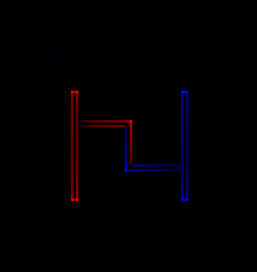
My answer is shown in figure 3. A number of simplifying assumptions have been made, notably the assumption that all the wires are small compared to the distance between wires. To obtain anything resembling a quantitatively-correct distribution would require FEM (finite-element modeling) software.

Figure 3: Charge Distribution in a Circuit

The ways in which this differs from figure 19.56 include:

• Within each segment of the large wire, let’s assume the capacitance per unit length is a constant. This is a lousy approximation, even in this simple circuit, and it is even worse for other circuits. Subject to this assumption, there is a definite charge per unit length for these segments.
• The charge per unit length on segment B is half the charge per unit length on segment A. Similarly the charge per unit length on segment D is half the charge per unit length of segment E. We know this by applying the voltage-divider formula (which is a corollary of Ohm’s law) to find the voltage, and then applying basic notions of capacitance.
• The charge per unit length on the fine wires is much smaller, because the self-capacitance is much smaller. The charge per unit length is so small it cannot be represented using the same scheme as the other charge densities. Let’s be clear: Even if we pretend the capacitance per unit length is constant for any given diameter of wire, it cannot possibly be independent of diameter.

As discussed in item 115, part of the problem is that the text speaks of «surface charge density» whereas the diagram depicts charge per unit length. These quantities differ by a factor of r. When we have wires of different r, the analysis given in the book is wrong. Indeed at this point we are two jumps removed from a reasonable analysis, because even if we took r into account, we would still suffer from the unreasonable assumption that capacitance per unit length is independent of the surroundings.

For sufficiently simplified surroundings, you can have a definite capacitance per unit length, but this has negligible practical or pedagogical value. It is misleading, because it is not representative of what happens in ordinary real-world circuits.

117.

The run-on sentence that makes up most of the final paragraph on page 778 is both ungrammatical and illogical. It seems that the topic of the sentence is going to be weight, but then it mostly talks about distance. This sentence really needs to become two sentences, possibly even two paragraphs.

118.

On page 793, and indeed throughout chapter 20, there are crucial limitations on the validity. Alas, these limitations are not stated, or even hinted at. As a result, many of the statements are not reliably true. This is an instance of the overall “limitations” issue discussed in section 2.1.

Specifically:

• At the start of section 20.1, the first paragraph needs to be removed. Most (perhaps all) of its content could be discarded entirely, since it is duplicative of the later discussion. Anything that needs to be preserved could be worked in later, about three paragraphs down the page. It cannot stay where it is, because it depends on assumptions, limitations, and provisos that have not yet been introduced.
• Then, the section needs to start by saying “Let us consider the scenario shown in figures 20.1 and 20.2’ or words to that effect. My point here is that much of what follows is true in that scenario but not reliably true otherwise.
• Even within the scenario, additional specificity is required. It needs to say “We have chosen the type of light bulb, the type of battery, and the type of capacitor so that the light bulb remains lit for several seconds before gradually dimming out.” My point is that this is a choice, not a law of physics.
• In the discussion of time scales, in the paragraph that straddles the bottom of page 793, it speaks of any «circuit containing a capacitor». This needs to be much more restricted. It should be restricted to the circuit in this scenario.

  (The contents of the paragraph that was removed can be worked in here, to the extent that they need to be worked in at all.)

• Last but not least, to show the boundaries of the primary scenario, contrasting scenarios should be mentioned: (A) If a smaller capacitor were used, the bulb would stay on for less time, perhaps many orders of magnitude less. (B) For a physically larger circuit, such as a lightning bolt or a nationwide power-distribution grid, it would take more than a few nanoseconds for the charge distribution to settle down, perhaps orders of magnitude more. (C) If we were interested in finer details of what is going on, for instance in the circuits inside a computer, where the switches are opening and closing billions of times per second, it would not be safe to assume that the settling-down timescale is short compared to other timescales of interest.

119.

On page 795, it speaks of «Charging a Capacitor». It must be emphasized that as a matter of terminology, this is absolutely not the same as “charging” a comb, or even “charging” one plate of a capacitor. When necessary, I use different terminology, namely gorging and disgorging a capacitor. An amount of gorge G on the capacitor as a whole corresponds to a charge Q₁ = +G on one plate of the capacitor and a charge Q₂ = −G on the other. Strictly speaking, the total charge Q is zero, since Q = Q₁ + Q₂ = 0 ... even though the gorge G is nonzero. See reference 27.

According to the laws of physics, it is perfectly possible to have the same sign of charge on both plates of a capacitor, for instance if you set the capacitor on top of a van de Graaf generator. The tradition in introductory engineering courses, as expressed by Kirchhoff’s laws, is to assume this cannot happen. However, the whole theme of chapter 20 and several other chapters is to connect the actual laws of physics to macroscopic circuit behavior. Using the same word, without explanation, for «charging» the capacitor as a whole and «charging» one plate of the capacitor pulls the rug out from under this effort.

In the real world, it is quite common to observe violations of Kirchhoff’s laws.

One cannot expect students to figure this out on their own.

120.

In about 20 places on pages 802 through 805, the absolute value bars around ΔV are quite wrong. In reality, if the voltage drop changes sign, the current changes sign (and vice versa).

The absolute value bars are not even used consistently. One example where they are not used is in the sidebar on page 803, where it claims «we always write ΔV = I R». On page 821, equation 821.60(R) omits the absolute value bars, while on the very next line, equation 821.63(R) has them. There are many other examples of this inconsistency.

121.

On page 807, the absolute-value bars in equation 807.16 and in equation 807.28 are quite wrong. Power can be positive or negative.

Also, writing it in terms of finite differences is silly; see section 2.4.

122.

On page 827, the absolute value bars in 20.P.59(a) are quite wrong. This stands in contrast to the definition of capacitance on page 799, where the bars are correctly absent.

123.

On page 839 it says «A compact device for creating such large potential differences is the “cyclotron.”» Alas the term “potential differences” is incorrect here. The cyclotron imparts a large energy to the particle, but it does not do it by means of a correspondingly large potential difference. In fact the cyclotron imparts kinetic energy to the particle, not potential energy.

Of course, in accordance with the “pseudowork / kinetic energy theorem” the cyclotron must have done work on the particle, but this is just another illustration of the fact that work is not a function of state. Work is not a potential.

I know that folks in the field measure every energy in electron·volts, but that’s just dimensional analysis; it does not mean there is a voltage anywhere equal to the total energy divided by e. Also the book treats voltage as synonymous with potential difference, but that is a profound misconception; in fact, not every voltage is a potential. So we are at least two jumps removed from equating the energy to a potential difference.

Simple suggestion: Just say “imparts energy” rather than “creates a potential”.

124.

On page 851, the discussion of «Non-Coulomb Work» is messed up in so many ways that one hardly knows where to begin.

1. Perhaps most importantly: There is absolutely no way a static magnetic field can do work on a point charge. This is a famous theorem. It is easy to understand and easy to prove. Hint: The force is perpendicular to the velocity.
2. Let’s look at equation 851.80. I assume all the quantities this equation are scalars, in accordance with the notation used throughout the book. Now, suppose you write out the corresponding vector equation, involving things like v→×B→. Then we can easily see that equation 851.80 is nonsense. The v in this equation is the speed of motion of the bar, as it moves in the x direction ... whereas the physically-correct equation would use the speed of the electron. Note that if it is to have any chance of moving from one end of the bar to the other, the electron must have some velocity component in the y direction. This y-velocity turns out to be a crucial part of the right answer.
3. When we consider conservation of energy, we find yet another difficulty. Energy must be supplied to the system from some external source, by something pushing on the bar. This is a force in the x direction ... even though the force implicitly implicated in equation 851.80 is in the y direction.
4. Equation 851.80 can be thought of as the right answer to a different question. There is in fact a voltage v B L between the two rails. It becomes an interesting physics question why an utterly wrong derivation produces a correct formula for the voltage. It’s probably just dimensional analysis in disguise; you can mention wrong physics or no physics at all, and still obtain equation 851.80 (or something similar) by dimensional analysis.

   We have several non-wrong ways of knowing the voltage:

   • Dimensional analysis tells us that v B L must be at least roughly right.
   • The Faraday-Maxwell law of induction says V = dφ/dt. The voltage is the time derivative of the flux.
   • If you insist on doing the calculation in the lab frame, the true physics involves at least two additional steps that page 851 does not even hint at. (On the other hand, the exceptionally astute student might realize that the argument on page 848 could be applied – in reverse – to shed some light on this problem.)
   • The elegant way to proceed is to transform into a frame comoving with the bar. When projected onto this frame, the electromagnetic field bivector has a component of the type conventionally called an “electric” field, even though the same electromagnetic field was purely magnetic when projected onto the lab-frame axes. It is easy to see how this E-field does just the right amount of work on the electron. For more on this, see reference 28.

     As a second step, you can calculate the y-motion and the associated force. This is proportional to the current. It is easy to see that the external push on the bar must be proportional to the current (among other things).

125.

On page 906, the section title asks «Law or Theorem?» This question is asked but never answered. Actually, I don’t want an answer, because the question should never have been asked in the first place.

The problem is that question implies that there might be an important difference between laws and theorems, which is a phenomenally bad idea. It is quite widespread, but that does not make it any less bad. This is discussed in reference 29.

126.

On page 917, figure 22.45 creates a very strong impression that the field vectors spiral outward, rather than pointing along the field line as they should. This is a manifestation of the issue discussed in section 2.8.

127.

On page 948 it says «the source of both the time-varying magnetic field and the curly electric field is varying (nonconstant) currents». Where’s That From? It’s not true. It’s particularly obviously not true for a radiation field propagating through a region of space where there no charge and no current.

128.

In this same paragraph on page 948, i.e. paragraph about «“magnetic induction”», the main point of the paragraph is seriously open to misinterpretation, because of the way it uses the word «source». It doesn’t actually say “cause” but many students are going to read it as a statement about causation ... which is a profoundly wrong idea. It doesn’t help to replace the traditional source (aka cause) with a more modern one, if the whole concept is wrong. See reference 4.

The correct concept goes something like this: It is somewhat misleading to say that the time-varying magnetic field “induces” the curly electric field, because Faraday’s law could equally well be interpreted as saying the curly electric field “induces’ the rate-of-change of the magnetic field.

129.

In this same paragraph on page 948, explaining «varying» in terms of «nonconstant» is completely pointless. If you mean time-varying, you have to say time-varying. Otherwise it could be varying (nonconstant) as a function of position alone.

130.

Let’s talk about the worked example that starts near the bottom of page 974, «Two Competing Effects in a Shrinking Ring». Borrowing the term «authentic» from reference 30, we can say that this example needs to be fixed, because it is inauthentic as it stands.

In the real world, devices like this actually exist and are used to trap and compress magnetic field lines. An example is described and analyzed in reference 31. This a ring with a high-enough conductivity, together with a short-enough timescale. There is no need for a separate, artificial, inauthentic statement about the rate-of-change of the magnetic field. The magnetic flux lines are trapped and therefore the magnetic field strength inside the ring is inversely proportional to the area. It’s just that simple. You can make it more complicated if you want, but there’s no need to.

So, by slightly changing the example from the book, we can make it easier to analyze, more interesting, and more authentic. It becomes a powerful lesson about the reality and utility of magnetic field lines.

To say the same thing the other way, if you thought of the magnetic field only in terms of a lattice of little arrows, it would be much harder to understand how such a device works. You would be likely to arrive at the inauthentic analysis that appears in the text.

As another argument leading to the same conclusion: The example in the text says the ring is «metal» but then ignores its electrical conductivity! This is weird, to say the least. As it stands, the example is ill-posed i.e. overdetermined. The inconsistency can be resolved in either of two ways:

If the intent was for the ring to be made of metal, it would have been better to not dictate the time-dependence of the field.

If for some reason you really wanted to impose a specified field, it would have been better to use a stretchy rubber ring, rather than a metal ring.

This is an instance of the larger issue discussed in section 2.6.

131.

On page 1011, the discussion of why the sky is blue mentions part of the explanation, but it is so incomplete as to be wildly misleading. In particular, it makes no mention of density fluctuations. If the atmosphere had a locally uniform density, the sky would be black, because atomic scattering would have no net effect, as we can understand (roughly) in terms of the Huygens construction. This has been understood for more than 100 years. See reference 32.

132.

There are numerous problems with the index. See section 3.

2  Big Issues and Recurring Themes

2.1  Limitations on the Range of Validity

By way of analogy, consider the two statements:

If you are going to teach people that a²+b²=c², you have an obligation to tell them that the result is valid for Euclidean right triangles only. This is important, because there are lots of triangles in this world that are not right triangles ... and lots that are not Euclidean.²

I mention this because this book contains a great many statements and equations that are perfectly true in context, but provide no hint as to the limitations on their validity. See e.g. item 17, item 66, item 74, item 75, item 91, item 101, item 114, and especially item 39 and item 118.

This is important! This is at least as important as anything else in the book. The primary, overarching objective of the course, as I see it, should be to teach students to think more clearly. That includes, among other things, recognizing the difference between (a) something that is true in all generality, as a fundamental principle of physics, and (b) something that is true in such-and-such scenario, because we chose to make it true.

It would help to remind students, more than once, that in physics, engineering, and everyday life, it is necessary to make approximations. It requires effort, skill, and judgment to tell the difference between a good approximation and a bad approximation. An approximation that works well in one situation might be disastrous in another situation. This is relevant because things that are exactly true (by hypothesis!) in a scenario might be only approximately true in the real world ... so there is a fine line between scenarios and approximations.

I don’t care very much whether students learn this-or-that specific physics fact. I care a great deal whether they learn to think clearly. See reference 33.

In the book, for instance in chapter 20 (item 118), one should not assume that the students will be able to sort out which statements are fundamental laws of nature and which are merely details of the scenario. Students were not born knowing how to do this. Also, one should not assume the teachers who adopt the book will emphasize this. If the book doesn’t emphasize it, why should they?

2.2  “Matter” versus “Interactions”

The “brand name” of the book is derived from the notion that all of physics can be categorized as either matter or interactions. Alas, this notion cannot possibly be true. This conclusion is supported by multiple lines of reasoning, all based on simple physics, including the following:

1. The emphatic assertion that «Interactions cause change» is problematic, as discussed in item 6.
2. We know from high-school chemistry that the mass of the helium atom is not equal to the mass of two protons, two neutrons, and two electrons. This is tabulated on the typical periodic table. There is a mass deficit associated with the binding energy. Therefore the “matter” we call helium includes the interactions in the nucleus. The same goes for every other element.
3. I’m trying to teach students about the unity and grandeur of physics. This is not made any easier when the book spends a large part of chapter 1 trying to de-unify things that have been unified for almost 90 years. I’m referring to the insight of de Broglie (reference 34), which was one of the all-time great breakthroughs.
4. Light deflected and/or redshifted by the gravitational field of a star – or galaxy or whatever – is an example of matter interacting with an interaction, which is quite inconsistent with the definitions given in the book.
5. Consider the apparatus shown in figure 4, which is based on Fig. 17-5 in Feynman volume II. The explanation is presented at the end of chapter 27-6; see reference 35. This is another example of matter interacting with a field, i.e. matter interacting with an interaction. Again this is inconsistent with the definitions given in this book.
   
   Figure 4: Momentum in the Fields
6. At many points, the book talks about the “Coulomb interaction” between two charged particles, so that there are two things and one interaction. In contrast, the modern (post-1864) way to think about the situation is to say that charge #1 couples to the field, and them sometime later the field couples to charge #2, so that there are three things and two couplings. The field is just as real as the two particles. This is a vastly better model of the physics. For one thing, it gives us a model that has no “action at a distance”, so it can be consistent with relativistic causality. It also gives us a model that treats all electric fields on the same footing, including the contributions from particles as well as the contributions from moving and/or changing magnetic fields. To calculate the electrical force on a test charge, all you need to know is the electric field; there is no distinction between the so-called Coulomb field and non-Coulomb field.

   This is relevant to the bar moving in a magnetic field, which is wrongly analyzed on page 851 of the book; see item 124.

   This may also be relevant to the profoundly wrong energy-based “explanation” for Kirchhoff’s voltage law, which is hinted at on page 751, explicitly emphasized on page 768, and repeated numerous times. See item 101. I conjecture that devotion to the notion of «mattter interacting with matter» could interfere with the concept of matter interacting with non-matter, such as particles that absorb energy that had been stored in a field. This particle/field concept is handled correctly on page 1003, but it is seriously mishandled in connection with Kirchhoff’s voltage law (page 751) and elsewhere.

7. Kinetic energy must be classified neither as matter nor as an interaction, AFAICT, according to the ordinary meaning of the words.
8. Advection must be classified both as matter and as an interaction, AFAICT. It satisfies the definition of interaction given on page 48, although it is omitted from the list of “interactions” on page 3. In one of the examples (I forget where), refueling is explicitly cited as a possible way of transferring energy. There are various possibilities, some of which clearly must be classified as matter:
   • Suppose object #1 emits a photon that is absorbed by object #2. This is a classic example of an interaction between two objects, right?
   • Now suppose object #1 emits an alpha particle that is absorbed by object #2. Is that the same thing or not? Is an alpha particle an object, or is it an interaction?
   • Further suppose some water evaporates from object #1 and condenses onto object #2. Is that the same thing or not? Is water matter, or is it an interaction?
9. The physics of a mechanical harmonic oscillator is isomorphic to the physics of an electrical LC oscillator, where L plays the role of the mass, and C plays the role of the spring ... or vice versa! You can equally well let L play the role of the spring, while C plays the role of the mass. So, in the electrical case, which is the “matter” and which is the “interaction”? The question is unanswerable – which is OK, because the question should never have been asked in the first place.

As a general principle, note that it is fairly common to have two names for the same thing. For lunch I had chickpeas seasoned with coriander ... which is exactly the same thing as garbanzos with cilantro.

Bottom line: The physics is what it is and does what it does. Trying to divide the physics into “matter” and “interactions” is not helpful, because it is not an apt model of the actual physics.

This has been known in the literature for a long time. The basic idea goes back to de Broglie. See also e.g. reference 36, which mentions the “electron field”.

2.3  Needless Radicalism and Needless Archaism

Note the inconsistency:

Authors should be free to choose whatever approach they like, within reason ... but please let’s not pretend there is any consistent policy behind these choices.

2.4  Finite Differences versus Calculus

On page v, the preface explicitly states that this book can be used in a course where calculus is a co-requisite rather than a pre-requisite. Therefore it would make sense to avoid calculus concepts (and calculus notation) in the early going. However, consider the following contrast:

It seems weird to use calculus on page 125 and then avoid it 500 pages later.

This is not the only example. There are multiple places where the book implicitly assumes that Δy/Δx must be synonymous with dy/dx. See item 73 for an example. Indeed on page 71 this is expressed explicitly; Under the heading of «Why Not Just Use Calculus?» it says «we actually are using calculus». On the next page it backs away from this slightly, saying that the finite differences are an «approximate evaluation» of the calculus result. Still, in any case, I must insist that «approximate evaluation» is not the same as equivalence, especially when supposedly fundamental principles are being expressed, such as on page 49; see item 17.

This is a time-dishonored swindle. Reference 37 discusses an example where Newton used this swindle. There are lots of things that are true in the limit that are simply not true for finite differences. In almost all cases, using the finite differences introduces some errors. If you want to argue that the errors go away in the limit, you have to actually make the argument. We know the result cannot be taken for granted, because:

• Among other things, you have to say you mean to take the limit, and then you have to demonstrate that the limit converges. Anybody who has ever done numerical integrations using finite differences knows that sometimes the limit converges very slowly ... and sometimes it doesn’t converge at all.
• There is also a huge body of mathematical theory about what you can do with limits and what you can’t. A lot of things that “look” like they ought to exist as physically-significant limits actually do not.
• As discussed in item 22, in the context of computer programming, there are places where the text throws around the symbol Δ with inconsistent meanings. These inconsistencies go away in the limit as Δ goes to zero, but they don’t go away in this situation. That’s because computer programs operate on finite differences and simply cannot pass to the limit as Δ goes to zero. If the inconsistencies in the text are not resolved in just the right way, program performance will be significantly degraded.
• Et cetera.

2.5  Great Man Theory

All too often, people who have not thought about the history of science attribute to Newton all sorts of ideas that that were figured out by Galileo and others. Similarly they attribute to Einstein all sorts of ideas that were figured out by Galileo, Lorentz, Poincaré, Minkowski, Debye, and others.

This may be a consequence of “Great Man Theory”. This is a completely discredited theory.

Wrongly assigning credit is not a trivial matter. The idea that it is OK to wrongly assign credit causes serious real-world problems, as discussed in reference 38.

I mention this because of things like item 4, item 5, item 9, and item 10.

2.6  Field Lines, or Lack Thereof

2.6.1  Virtually No Field Lines In the Book

I cannot find any pictures of electric field lines or magnetic field lines anywhere in the book, even in situations where such a picture would be traditional and helpful. See e.g. item 79. This is intentional, as the authors explain in reference 30.

This seems odd. The concept of field lines has been around a very long time, longer even than the Maxwell equations. In four dimensions the concept works rather well. In three dimensions the concept is imperfect, but sometimes an imperfect picture is better than nothing. In any case, the concept is far less imperfect than some of the things that do prominently appear in the book, such as the lattices of little arrows that are used to represent the field.

2.6.2  An Example of Field Lines

By way of contrast, to get a feeling for the value of field lines, take a look at figure 5.

Figure 5: Field Lines of a Loose Solenoid

There is a tremendous amount of information in this figure. As far as I can tell, there is no way to convey more than a tiny fraction of this information using a lattice of little arrows.

Let’s be clear: A lattice of little arrows does have some value. As I see it, its primary value is as a preliminary step, as an aid to drawing the field lines!

Besides, figure 5 is just plain pretty. It’s much prettier than a lattice of little arrows.

2.7  The Topology of the Field is Important

There are some places where the book tries to make a point about the global structure of the field, such as figure 18.33 on page 725. Alas, the book insists on representing the field using lattices of little arrows. The problem is that the arrows are disconnected and too few in number to permit the student to visualize the topological structure of the field.

This is a nontrivial matter. The statement ∇·B=0 has a rather profound topological interpretation. Similarly for ∇·E=0 in empty space. Specifically, on page 560, the field is divergence-free except at the origin, but this is not the least bit obvious from the diagram.

One place where there are almost enough arrows to show the structure of the field is figure 23.3 on page 949.

Ironically, another one of the few places that has a dense-enough distribution of arrows to permit some discussion about the topological structure of the field is in figure 17.85 on page 706. This is ironic because it is intended to illustrate a situation that cannot exist (not within electrostatics, anyway).

Another issue pertaining to the topological structure of the field is discussed in section 2.8.

2.7.1  No Equipotentials, Either

Additional information about the topological structure of the field can be represented by equipotential contours. As far as I can tell, the book doesn’t do this either. The word “equipotential” does not appear in the index or table of contents, and google cannot find it anywhere in the book. Similarly, apparently it does not appear anywhere in reference 30.

The lattices of vectors that do appear in the book cannot be used to visualize the equipotential contours in any natural way.

The arguments in reference 30 about the problems with drawing field lines in two dimensions (for instance, in connection with an electrically charged ring) do not apply to drawing equipotential contours.

As a related matter: I reckon students should know how to interpret the contours on a topographic map. If they don’t already know, it’s high time they learned. This can be used as an example of physics in the real world, as an example of the unity of physics. The contours on the topo map are equipotential contours of the gravitational potential.

At this point we can spiral back to the definition of vector. As discussed in reference 25, there are actually two kinds of vector: pointy-vectors and one-forms. Column vectors and row vectors. Kets and bras. The closeness of the contours on a topo map, or on a plot of the electrostatic potential, is an excellent representation of the gradient vector, represented as a one-form rather than as a pointy-vector. This is important for innumerable applications, including maps, electromagnetism, thermodynamics, quantum mechanics, et cetera.

2.7.2  The AJP Article

The arguments in reference 30 are very incomplete and unbalanced. They fixate on the costs of dealing with field lines and wildly underestimate the value.

The article proves that field lines should not be handled in a dumb way, but comes nowhere near proving that they should not be handled at all. It proves that they can be handled badly, but does not prove that they cannot be handled well.

Field lines have a profound a topological significance, namely the continuity of the field lines. Drawing a bunch of little arrows here and there is nowhere near sufficient to portray continuity.

In section VI, the AJP article talks at length about all the things that can go wrong if topology is not handled correctly, but it quite unfairly downplays the value. The idea is all the more valuable because it applies to lots of things, not just field lines. The foundations of physics, namely the conservation laws, are essentially topological, insofar as they express the continuity of world-lines. Note that topological continuity can be expressed directly, in pictorial terms, long before students know enough math to do quantitative calculations using Gauss’s law.

The AJP article contains many arguments against field lines, but many of the arguments are not as strong as they might at first appear.

• We agree that the “typical” textbook treatment is terrible. However, there is nothing special about this. The same problem affects mechanics (e.g. monkey-shooting) but we do not respond by tossing mechanics out of the curriculum.

  There is a proverb that says no matter what somebody is doing, he can always do it wrong ... but that does not mean that we are obliged to make all the same mistakes.

• We agree that if you have an electrically charged ring, it is not possible to draw the field lines in 2D. However, once again, there is nothing special about that. The very cover of the book features a diagram that could not have been drawn in 2D. We do not respond by throwing all such diagrams out of the curriculum.
• The ⊗ and ⊙ symbols in the figures on pages 850 through 853 (and elsewhere) are for practical purposes a view of a transverse section of the field lines. The density corresponds to field strength.

  So the book does not entirely uphold the “principles” espoused in the article.

• We agree that students have a hard time drawing the correct field lines by hand. However, it’s also hard for them to draw the correct lattice of little arrows by hand, especially in 3D.
• Again, we agree that students have a hard time drawing the correct field lines by hand ... but that is beside the point, several times over. Forsooth, it’s hard for experts to draw the correct field lines by hand. That’s what computers are for. Note that figure 5 was prepared using free, open-source software.

  Again, there’s nothing special about this. It’s hard to draw decent graph paper by hand, so we don’t ask students to do that. We just give them graph paper.

  I can’t draw a detailed map of Africa by hand, but if somebody gives me a map I can interpret it. The idea of turning out students who don’t know how to interpret figure 5 is horrifying.

• It is an overstatement to say there is an «absence of authentic tasks» for homework problems. There may be a shortage, but not a complete absence. Furthermore, again, there is nothing special about this. Monkey-shooting is infamously inauthentic.

  I spent a few minutes thinking up some «authentic tasks»

  1. See item 130.
  2. Explain why the magnet in figure 6 has pole pieces shaped like frustrated cones.
     
     Figure 6: Laboratory Electromagnet

     This strikes me as at least as authentic as the circuit shown in Fig. 2 in the AJP article ... and also in figure 19.56 on page 778 of the book. Indeed you could use the very same diagram and replace the wire by a high-permeability material and replace the power-supplies by coils, and achieve more-or-less the same level of authenticity.

  3. The lift of a wing is best explained in terms of circulation, and the vortex lines obey the same equation as magnetic field lines. As a famous man once said, the same equations have the same solutions. The continuity of the vortex lines explains the origins of the wake vortex, which has tremendous real-world significance.
  4. At the hands-on level, get a big strong magnet and decorate the field lines with iron filings or iron powder. Let students /touch/ the filaments. This provides a 100% "authentic" perception of tension along the field lines and repulsion between field lines – two concepts that significantly predate the Maxwell equations.

     I’ve been doing that experiment since I was 4 years old. One might hope that all students would have done that experiment in grade school ... but many have not.

     This has 100% "authentic" applications in industry, including ferrofluidic rotating seals, and ferrofluids for visualizing data on magnetic media.

  5. Consider quantized flux lines in type-II superconductors:
     http://www.nobelprize.org/nobel_prizes/physics/laureates/2003/illpres/vortices.html
     http://www-personal.umich.edu/~nori/science_text.html
     http://physics.nist.gov/TechAct.2002/Div841/div841.html
     
     
     Figure 7: Flux Lattice

     This is not a hands-on activity, and the details of what’s going on are beyond the scope of the introductory course, but it does make for nice pictures. It is 100% "authentic" in the sense that the flux lattice is not an artist’s impression, and is not a simulation.

  6. There is an analogous vortex lattice in superfluid helium.
  7. Similarly, consider flux lines popping in a RF SQUID.

2.8  Vector Attachment

In figure 8 and similar diagrams, the following rules apply: The black arrows represent a vector field. For each arrow, the black circle tells which point in the field is being described by the vector. We call this the point of attachment. The length and orientation of the arrow tells us the magnitude and direction of the field at that point.

For figure 8 in particular, each vector is plotted in such a way that the point of attachment coincides with the midpoint of the arrow.

Figure 8: Velocity Vectors Attached at the Midpoint

Figure 9: Velocity Vectors Attached at the Tail		Figure 10: Velocity Vectors Attached at the Tip

The contrast is worth emphasizing:

1. In terms of fundamental physics, or rather mathematics, that all three of these diagrams represent exactly the same vector field. The field is being evaluated at the same six points, and at each point the direction and magnitude of the field is the same in all three figures. The locations of the black arrows mean nothing; only the magnitudes and directions are meaningful. (The locations of the points of attachment are meaningful, but the locations of the arrows are not.)
2. In terms of psychology and pedagogy, the three figures are very different. In terms of the art and science of “display of quantitative information”, the three figures are very different. At first glance it “looks” like the vector field in figure 9 is spiraling outward, and that the vector field in figure 10 is spiraling inward ... neither of which is an accurate perception.

   For most purposes, figure 8 is a much better depiction, insofar as it is easier to interpret correctly. In particular, suppose we are trying to depict a divergence-free field, such as a magnetic field or the flow of a conserved fluid. Figure 8 “looks” divergence-free. That is to say, it quite appropriately “looks” like the vector is just pulling you along a field line, with no tendency to pull you away from the field line.

I mention this because throughout the book, vector fields are plotted with the attachment points at the tails of the vectors. This makes some of the diagrams hard to interpret ... quite unnecessarily hard. See item 53 and item 126 for some conspicuous examples. Another example can be found on page 948, along with multiple examples on pages 949 and 950. Even the iconic diagram on the cover (figure 11) suffers from this disease.

Figure 11: Magnetic Field with Bogus Divergence

We see a similar phenomenon in the following figures, all of which are trying to present the same information. The true symmetry of the situation can be seen in figure 12 or, better figure 15, or even better figure 16. Figure 13 corresponds to figure 14.66 on page 580, and significantly distorts the symmetry, insofar as it makes it appear that the center of the figure is quite a bit higher than it really is. Figure 14 shows the opposite distortion.

Figure 12: Dipole Field Attached at the Midpoint

Figure 13: Dipole Field Attached at the Tail		Figure 14: Dipole Attached at the Tip

Figure 15: Dipole Field Rooted at the Midpoint

Figure 16: Dipole Field Rooted at the Midpoint, with Circle

Another issue pertaining to the topological structure of the field is discussed in section 2.6.

2.9  Bogus Absolute Value Bars

If you start with a correct equation and take the absolute value of one side, or both sides, you make the equation worse, not better. Also, when doing a calculation, taking the absolute value is not an acceptable substitute for calculating the correct sign.

I mention this because in many places throughout the book, there are absolute value bars where they don’t belong. Examples include item 13, item 99, item 121, item 122, and several of the errata in section 4.

A different sort of problem related to absolute values is discussed in item 90.

2.10  Regimentation Marches On

For his own use, the teacher (or the textbook author) is free to choose a reference frame – or a gauge – or a method of solution ... but other people are free to choose differently. Students are people too.

The teacher (or the textbook author) can even recommend a reference frame – or a gauge – or a method of solution ... but this should clearly be labeled as a recommendation ... not a law of nature. Other approaches should not be considered wrong.

Einstein said his teachers required Kadavergehorsamkeit ... the obedience of a corpse. Any sign of creativity or original thinking was ruthlessly suppressed. I’ve seen plenty of classrooms that still play by the same rules. They emphasize authority, conformity, and regimentation to the exclusion of almost all else.

I mention this because of things like item 32 and section 2.11.

2.11  Numbering the Equations

Apparently none of the equations in the book have equation-numbers. By all accounts, this is not an oversight. The authors are of the opinion that «it is a feature, not a bug».

Reportedly, the authors are worried about the following scenario: Some teacher is “lecturing from the book” and wants to refer to a particular equation. The authors wish to force him to write out the equation in full, rather than merely citing it by number.

I am astonished by the naiveté and utter futility of this wish. There is (at present) nothing stopping the teacher from citing “the second equation on page 56” – as the authors themselves do in the errata (reference 1). Another tactic is to cite “equation 670.42” which refers to the equation that is 42% of the way down from the top on page 670 – which is the technique I have used in these notes. Oh wait, my friend Simplicio has a suggestion:

In the next edition of the book, let’s remove the page numbers as well! After all, why should the teacher be allowed to cite the page by number? We can compel him to write out the page in full, rather than citing it by number, just as we compelled him to write out the equations in full. Similarly, we should de-number all of the chapters and diagrams. We can compel the teacher to re-draw each diagram in full, rather than citing it by number.   That will teach ’em a lesson. That will show ’em who’s important and who’s not.   Heaven forbid that Suzy Q. Student would want to tweet a question or a remark about one of the equations. How dare anyone try to use the book in a way that was not foreseen and approved by the authors? It’s shocking how uppity the riff-raff is getting.

3  Bugs in the Index

• In the index, the priorities are remarkably out of kilter. For example, in contrast to important concepts such as “Mass” and “Time” and “Laws of Motion” that are essentially not indexed, the bizarre and mostly-wrong «maximum-power engine» gets indexed at least four times
  • engine, maximum-power
  • engine, maximum power output
  • maximum-power engine
  • maximum power output
• The second law of motion is not indexed at all — not under “Second”, not under “Law”, and not under “Motion”. Oddly enough, it is indexed a couple of times under “Newton”, which is not much help, because it is not where users are going to look.
• The third law of motion is not indexed at all — not under “Third”, not under “Law”, not under “Motion”, and not even under “Newton”.

  The word “reciprocity” – which is used as a code-word for the third law – has only one entry in the index, and the referent is less than brilliant, as discussed in item 26.

• The concept of “Time” is not indexed at all.
• The concept of “Mass” is indexed only as «mass, hot object», plus «mass-spring system initial conditions» and «massles particles».
• «Momentum Principle, The» is indexed separately from «Momentum Principle».
• «gravitational forced» is indexed separately from «gravitational force».
• «force» is indexed separately from «forces».
• «non-Coulomb forces» is indexed separately from <non-Coulomb force».
• The indexing of «non-Coulomb electric field» is inconsistent with the indexing of «electric field, non-Coulomb».
• The Geiger-Müller tube on page 704 is not indexed.
• The indexing of Kirchhoff’s laws is very sketchy; it omits almost all of the places where they appear; see e.g. item 102. It even omits the place where they are introduced.
• Although the term “work function” is used in various places in the text, it is not indexed. A pointer to the definition would be helpful.
• Some index entries are simply wrong. How is this even possible, given that the index was generated by a computer? For example:
  • The index entry for «gravitational constant» points to page 98, even though this constant was introduced on page 96.
  • The index entry for «Conservation of charge» points to page 586, which is not the right page; 585 would be better.
  • The index entry for the «fundamental assumption of statistical mechanics» points to page 477, which is not the right page; 476 would be better.
• The first entry in the “Q” section has a body but no headword. Presumably the headword was meant to be Q itself, but it does not appear. Even if it did appear, it would look weird, because more-important quantities such as E, S, T, P and V are not indexed at all.
• The discussion of «why the sky is blue» is indexed under «why» – which is not where any reader is going to look. On the other edge of the same sword, if you’re going to index one thing under «why» there are innumerable other things that ought to be indexed the same way.

Suggestion: The authors (or the publisher) should hire somebody who knows what they’re doing to deal with the index. There exist professional indexers who specialize in science texts.

Workaround: You may be able to use Google Books to search for things you want. The google machines are obviously devoid of judgment, and will therefore never take the place of a well-crafted index, but it’s better than nothing.

Also note that google limits how much of the book you can see, and you can very quickly run up against this limit.

4  Errors in the Errata

This refers to the errata in reference 1.

• On page 19, after being corrected, the m inside the square root in the denominator needs to be m² ... or it needs to move outside the square root.
• In the erratum for page 24, 1.X.32: «Assume that the velocity is nearly constant for this rather short time.» That doesn’t work, because nobody plays baseball in a zero-g environment, and in half a second the velocity necessarily changes by a significant amount (in the ordinary terrestrial reference frame). It would be better to say that the specified velocity is the average velocity (not «constant» velocity).
• On page 271, after being corrected, I’m pretty sure it was supposed to be p₁ (subscript numeral 1) not p_i (subscript letter i).
• The proposed correction for page 304 is wrong; it should end in v not r.

  As a separate matter concerning this equation, see item 43.

• If you carry out the proposed correction for page 424, the result will have an ugly nonlocal link to «the previous exercise». It would be better to restate the conditions, or at least to link to the other exercise by number, explicitly.
• The proposed correction for page 541 is a Bad Idea. If you replace W with |W|, you get an equation that has two solutions, only one of which is correct. You could fix this by writing down additional equations, but it would be far better to leave off the absolute value bars and instead insert a minus sign in front of the W in equation 541.26. Compared to inserting absolute-value bars, this makes the equation simpler and more correct. See item 76.

  As for the observation that «In the later part of the page, W is an input to the system and is positive», the later usage is consistent with the definition of W in chapter 6 and elsewhere. However, equation 541.65 has other issues; see item 77.

  The book defines W := −∫P dV as we see on page 527 and elsewhere. This represents work done on the system by an external force. The book is commendably consistent about using this definition ... with the glaring exception of page 541. If you want to discuss work done by the engine, that’s fine, but it should be denoted −W, or perhaps by some other symbol entirely.

• Ditto for the proposed corrections on pages 544, 549, and 550. When doing calculations, throwing in absolute-value bars is not an acceptable substitute for getting the minus signs right.
• In the second erratum for page 550, the approved SI style is “0 ^∘C” (not «0^∘»).
• In the correction for page 697, it is not reliably true that the energy density has units of J/m³. I can choose whatever units I like, so long as they have the correct dimensions.

  Secondly, the field energy density is ½є₀E², period. Adding a factor of J/m³ makes the expression incorrect. You might have 13 J/m³, but not ½є₀E² J/m³. If you want to remark upon the dimensions of the energy density, you can do that, using words in a sentence ... not by simply tacking on extraneous factors of J/m³.

  If (J/m³) was meant to be a parenthetical remark, as opposed to a factor, it is very unclear and also inconsistent with every other equation on the page (and probably every other equation in the book). It would help to use actual words to say what you mean.

5  References

1.

“Errata for Matter and Interactions 3rd edition
http://matterandinteractions.org/Content/Errata/Errata_3e.pdf

2.

John Denker,
“Periodic Table of the Elements – Cylinder with Bulges”
www.av8n.com/physics/periodic-table.htm

3.

Rawlings “REACTBALL”
http://rawlings.com/product/reactball/REACTBALL(Rawlings)

4.

John Denker,
“Cause and Effect”
www.av8n.com/physics/causation.htm

5.

John Denker,
“Welcome to Spacetime”
www.av8n.com/physics/spacetime-welcome.htm

6.

John Denker,
“Decorated Symbols (e.g. x-bar, q-dot, v-vector) in HTML”
www.av8n.com/physics/decorated-symbols.htm

7.

John Denker,
“Definition of Weight, Gravitational Force, Gravity, g, Latitude, et cetera”
www.av8n.com/physics/weight.htm

8.

John Denker,
“Basic Properties of a Symplectic Integrator”
www.av8n.com/physics/symplectic-integrator.htm

9.

John Denker,
“Dimensionless Units”
www.av8n.com/physics/dimensionless-units.htm

10.

Benny Lautrup,
“Hydrostatic shapes”
http://www.cns.gatech.edu/~predrag/courses/PHYS-4421-10/Lautrup/shapes.pdf

11.

John Denker,
“Motion in a Rotating Frame”
www.av8n.com/physics/rotating-frame.htm

12.

John Denker,
“Modern Thermodynamics”
./thermo/

13.

John Denker,
“Visualizing A Field that is Not the Gradient of Any Potential”
www.av8n.com/physics/non-grady.htm

14.

Wikipedia article, “Macroscopic quantum phenomena”
http://en.wikipedia.org/wiki/Macroscopic_quantum_phenomena

15.

John Denker,
‘Coherent States”
www.av8n.com/physics/coherent-states.htm

16.

Michael G. Moore,
“Introduction to Scattering Theory”
http://www.pa.msu.edu/~mmoore/852scattering.pdf

17.

John Denker,
“Models and Pictures of Atomic Wavefunctions
www.av8n.com/physics/wavefunctions.htm

18.

John Denker,
“Quantifying Entropy” in chapter 2 of Modern Thermodynamics
www.av8n.com/physics/thermo/entropy.html#sec-quantify-s

19.

John Denker,
“A Fluid Has Pressure Everywhere”
www.av8n.com/physics/pressure-everywhere.htm

20.

John Denker,
“Power Plant Efficiency”’
www.av8n.com/physics/power-plant-efficiency.htm

21.

John Denker,
“Why White Things are White”
www.av8n.com/physics/white.htm

22.

John Denker,
“Contact Electrification”
www.av8n.com/physics/contact-electrification.htm

23.

John Denker,
“One Kind of Charge”
www.av8n.com/physics/one-kind-of-charge.htm

24.

Steven Weinberg,
The Discovery of Subatomic Particles Revised Edition

25.

John Denker,
“Introduction to Vectors”
www.av8n.com/physics/vector-intro.htm

26.

John Denker,
“How a Battery Works”
www.av8n.com/physics/battery.htm

27.

John Denker,
“Gorge versus Charge”
www.av8n.com/physics/gorge-vs-charge.htm

28.

John Denker,
“The Microscopic Origins of the Magnetic Field”
www.av8n.com/physics/magnet-relativity.htm

29.

John Denker,
A discussion of rules, laws, theorems, et cetera, in “Scientific Methods”
www.av8n.com/physics/scientific-methods.htm#main-rule-law

30.

Ruth Chabay and Bruce Sherwood,
“Restructuring the introductory electricity and magnetism course”
AJP 74, 329-336 (2006)
http://scitation.aip.org/content/aapt/journal/ajp/74/4/10.1119/1.2165249
http://matterandinteractions.org/Content/Articles/AJP-EandM.pdf

31.

Wikipedia article,
“Explosively pumped flux compression generator”
http://en.wikipedia.org/wiki/Explosively_pumped_flux_compression_generator

32.

John Denker,
“Why the Sky is Blue”
atom-intro.tex-www.av8n.com/physics/blue-sky.htm

33.

John Denker,
“Learning, Remembering, and Thinking’
www.av8n.com/physics/thinking.htm

34.

Louis de Broglie,
“Recherches sur la théorie des quanta” (PhD thesis, 1924)
http://tel.archives-ouvertes.fr/docs/00/04/70/78/PDF/tel-00006807.pdf

35.

The field momentum issue, as discussed in:
Feynman, Leighton, and Sands,
The Feynman Lectures on Physics
Question: http://www.feynmanlectures.caltech.edu/II_17.html#Ch17-F5
Answer: http://www.feynmanlectures.caltech.edu/II_27.html#Ch27-S6

36.

Frank Wilczek,
“Mass without Mass I: Most of Matter”
Physics Today (November, 1999)
http://scitation.aip.org/content/aip/magazine/physicstoday/article/52/11/10.1063/1.882879
http://ctpweb.lns.mit.edu/physics_today/phystoday/MassI.pdf

37.

John Denker,
“Kepler’s Equal-Area Law, Angular Momentum, and the Laplace-Runge-Lenz Vector”
www.av8n.com/physics/kepler-equal-areas.htm

38.

John Denker,
“Students Need the Best Evidence, Not the Most Ancient Evidence”
www.av8n.com/physics/best-evidence.htm

1

Note that I generally don’t write arrows over my vectors, except when quoting somebody else; see reference 6.

2

As the name suggests, geometry was initially the science of surveying the surface of the earth. However, the formula a²+b²=c² does not reliably apply to the surface of the earth, because the surface is curved, not planar. If you carefully survey a moderately large triangle, you will notice the curvature. Indeed, if you make the triangle large enough, you can construct on the surface of a sphere a triangle with three right angles.